Computation Is Not Integration

Integrated Information Theory (IIT) applied to artificial neural networks — exact Φ for small systems, and the scalable Gaussian Φ* proxy for recurrent networks during training.

1Overview

1.1Research question

Is there more to consciousness than computation? Integrated Information Theory answers yes: consciousness corresponds to a system's intrinsic, irreducible cause–effect power — quantified by Φ — rather than to the function it computes. Artificial neural networks let us examine that claim concretely, because a network's connectivity can be edited independently of the task it solves.

This project computes two quantities and keeps them rigorously distinct:

Exact Φ (IIT 3.0, via PyPhi) — the intrinsic, consciousness-associated quantity. Precise, but its cost grows as O(2ⁿ), so it is tractable only for very small systems.
Approximate Φ* (Barrett–Seth / Oizumi–Amari) — a scalable, Gaussian measure of dynamical integration. Φ* is not IIT's Φ and is not a measure of consciousness.

1.2Summary of results

A feedforward network classifies MNIST accurately yet has Φ = 0.
Rewiring the same-sized network for recurrence raises it to Φ = 2.47 — without changing the task.
Under a matched estimator the RNN/GRU/LSTM Φ* ordering reverses relative to the initial implementation.
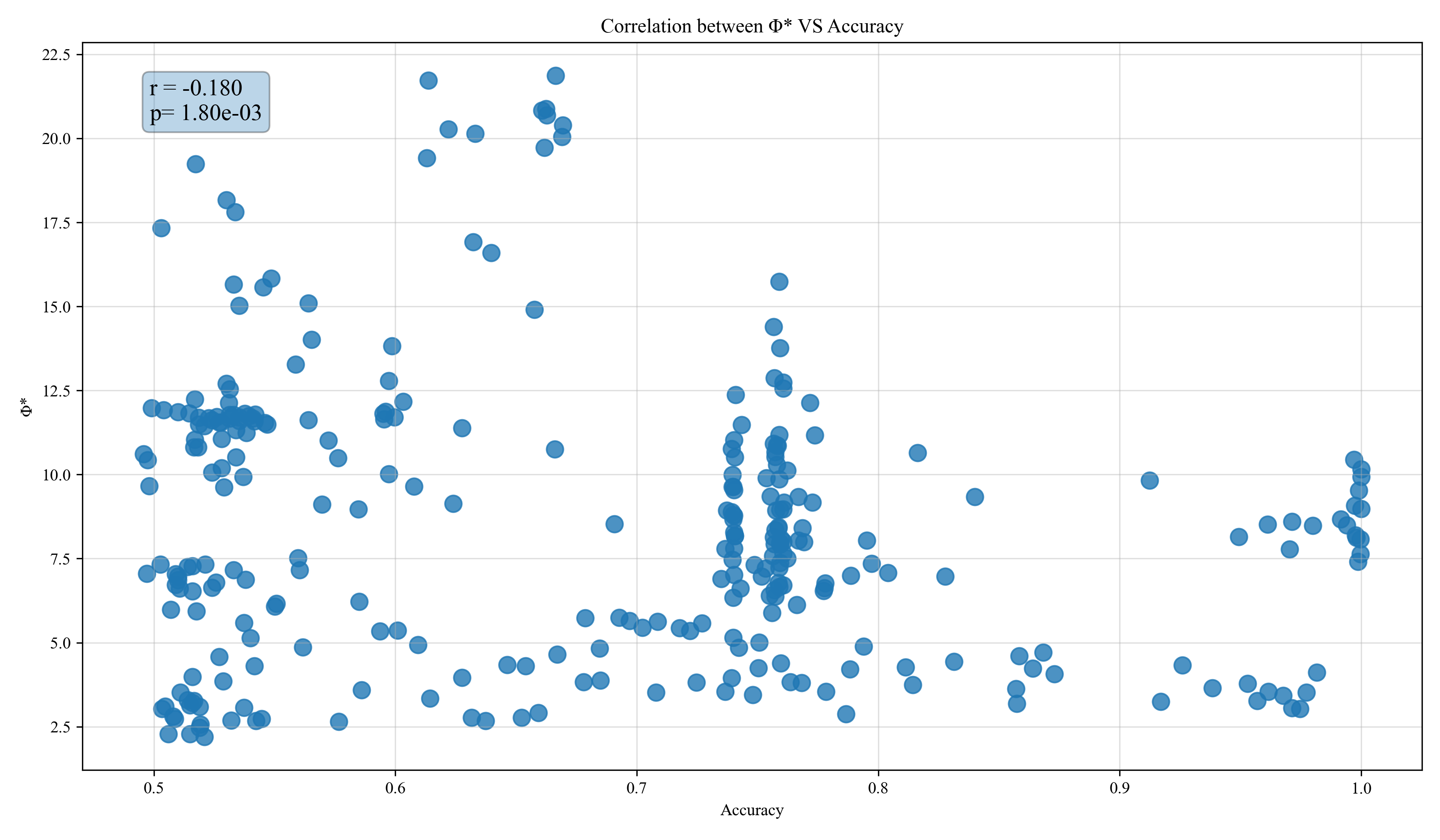
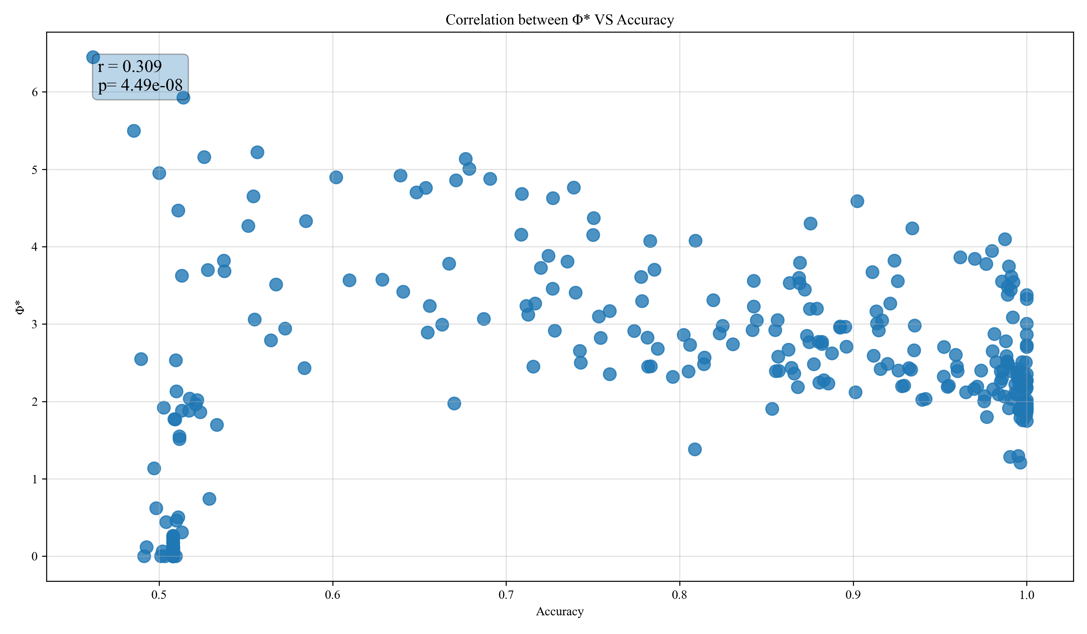
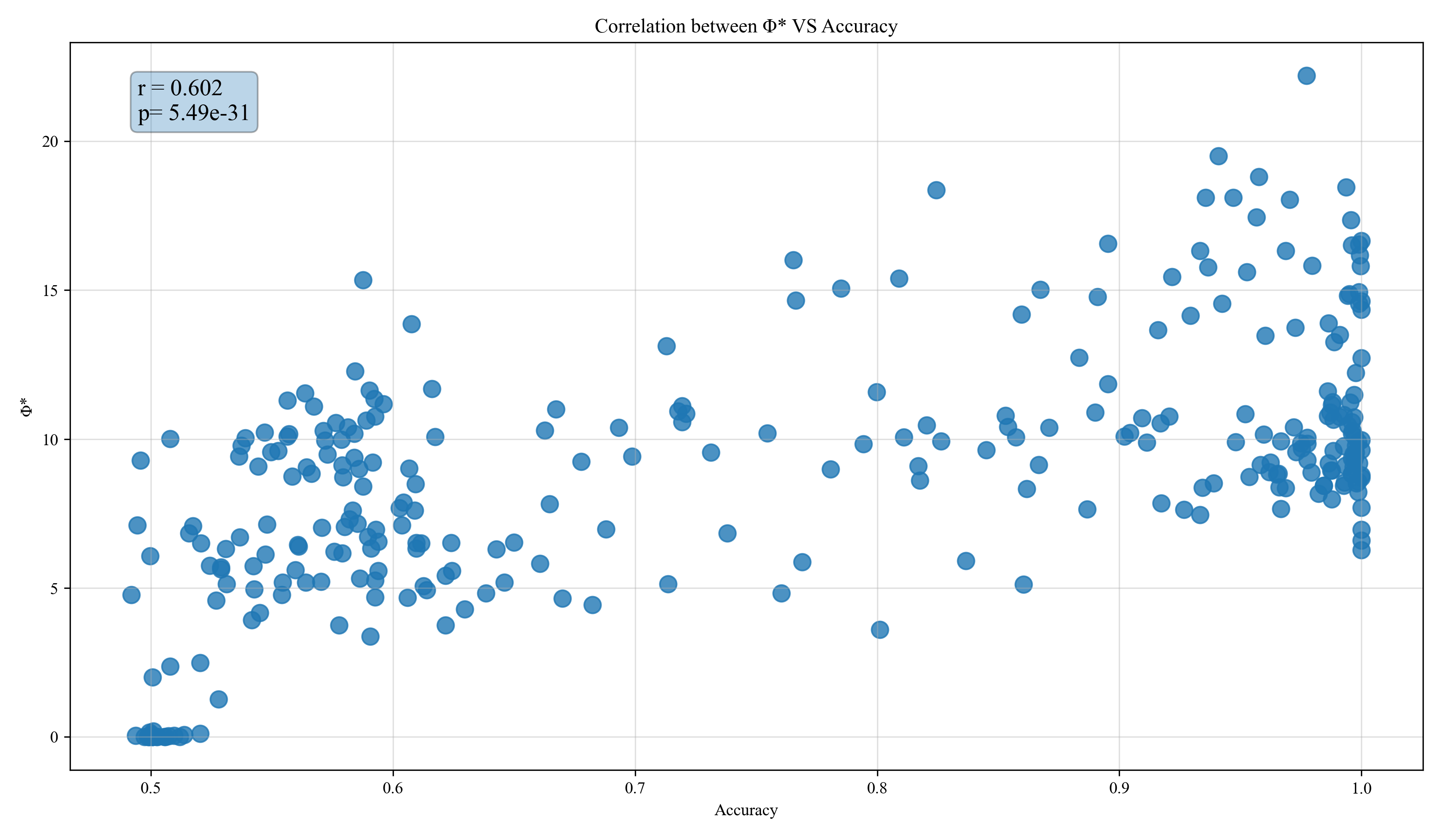
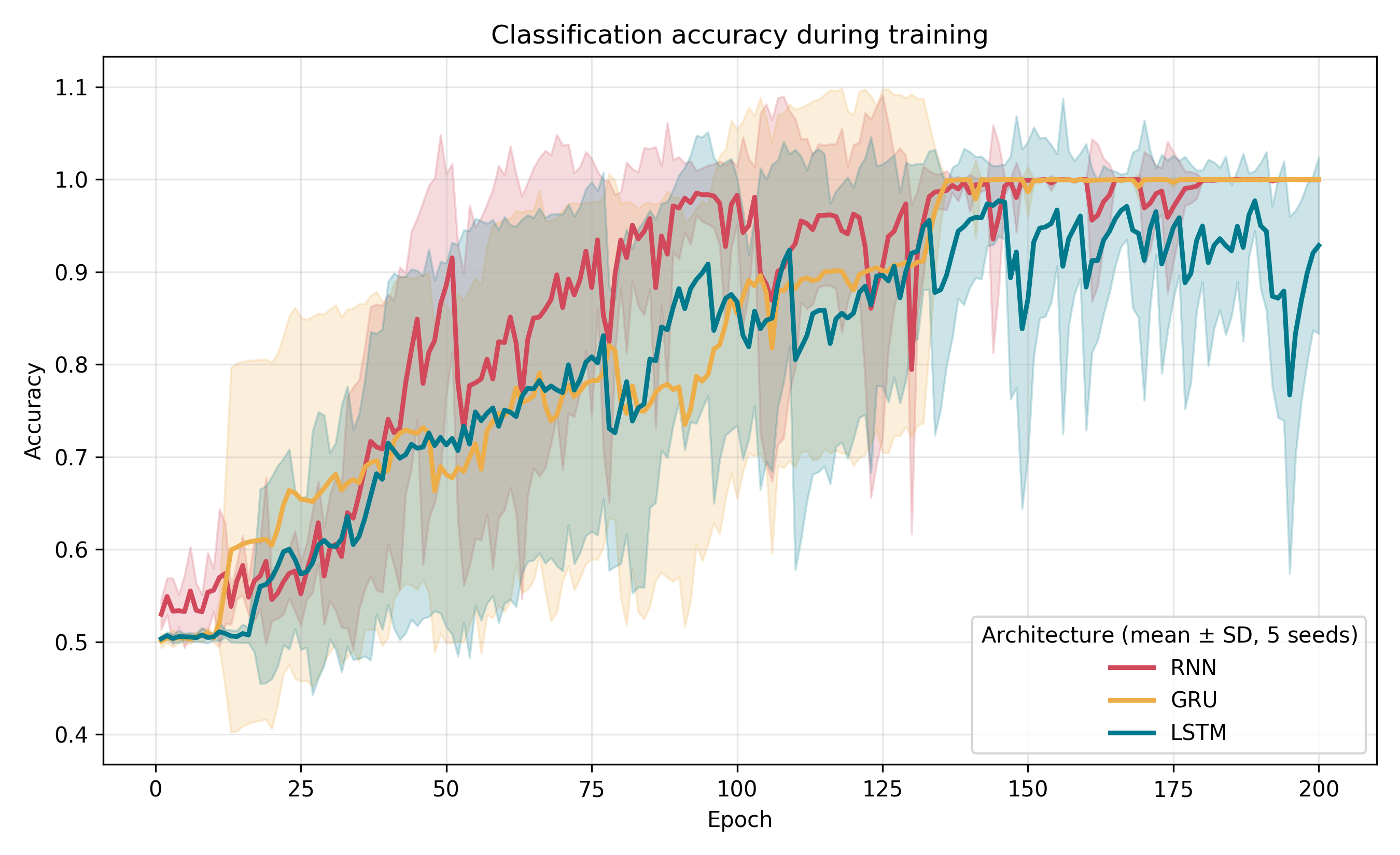
Φ* is statistically uncorrelated with accuracy: integration and computation are dissociated.
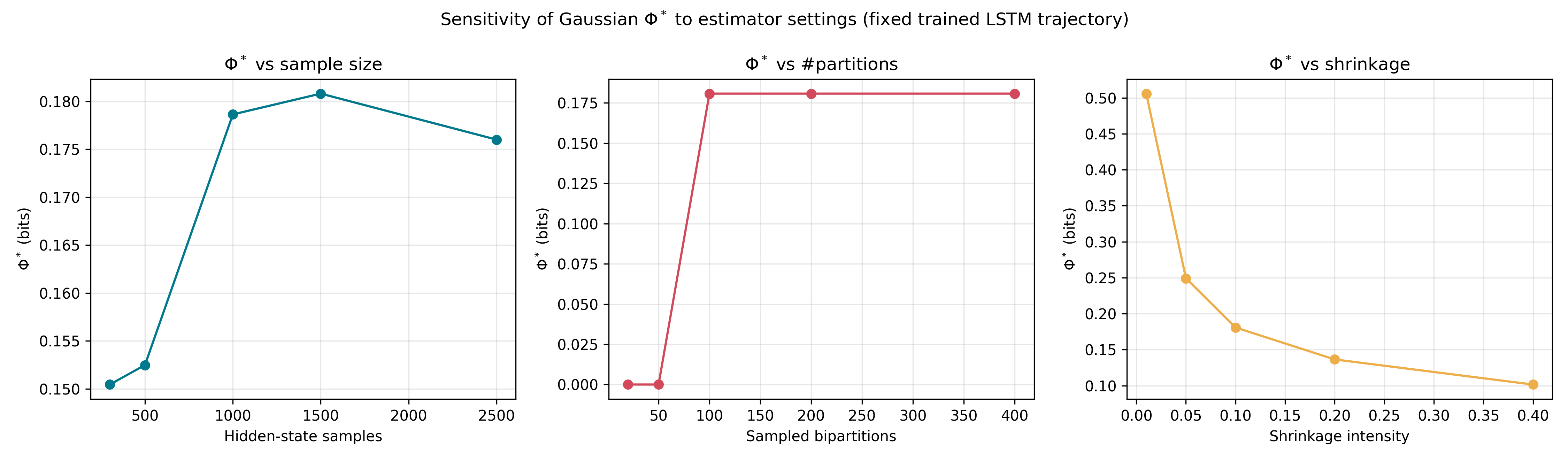
Φ* itself is highly estimator-dependent, with a non-zero floor.

No claim of machine consciousness is made. Under strict IIT every network studied here — running on a digital substrate — would have negligible intrinsic Φ. The contribution is methodological: a reproducible account of where measures of integration succeed and fail when applied to AI.

2Background

2.1Axioms and postulates

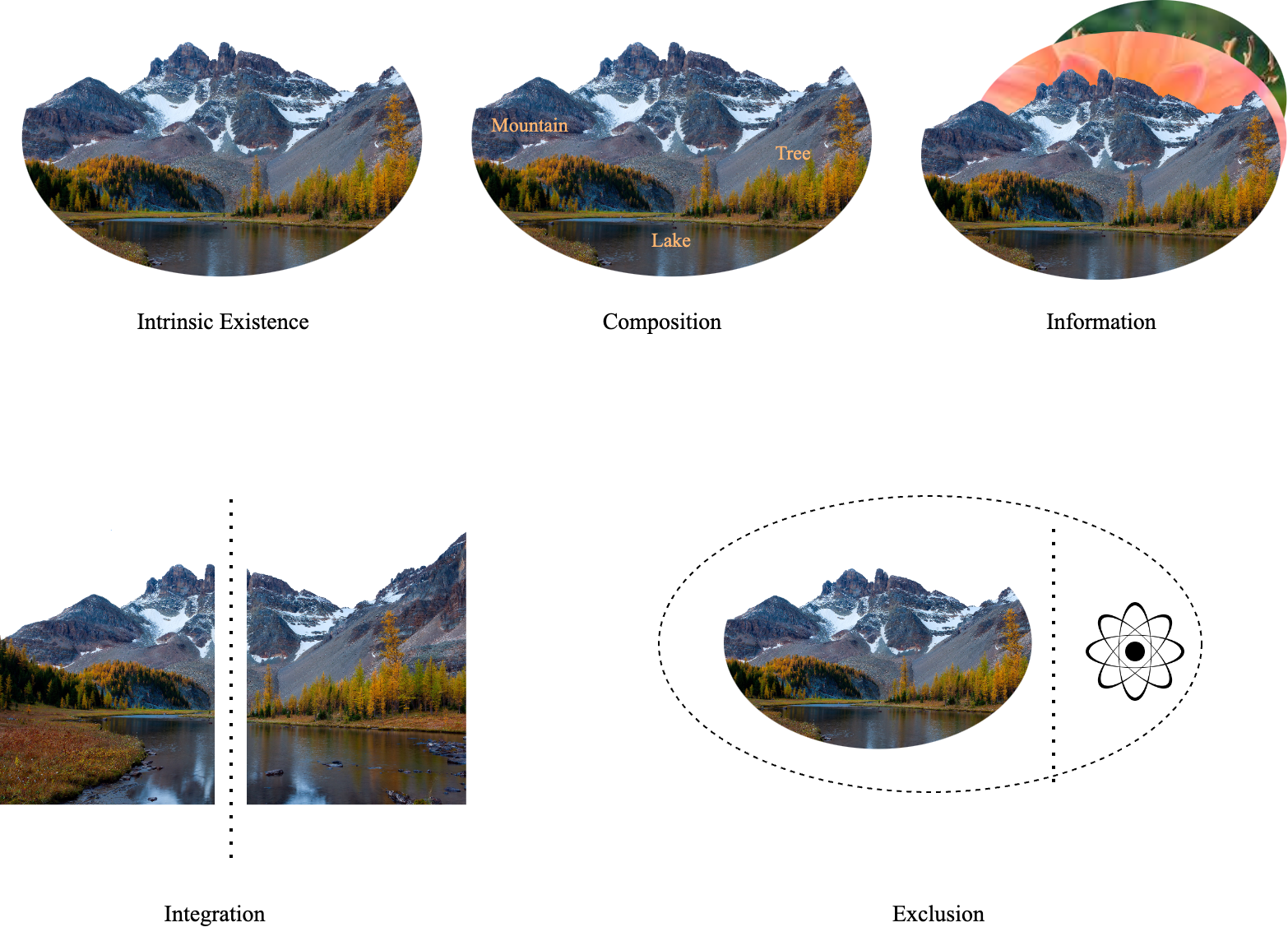
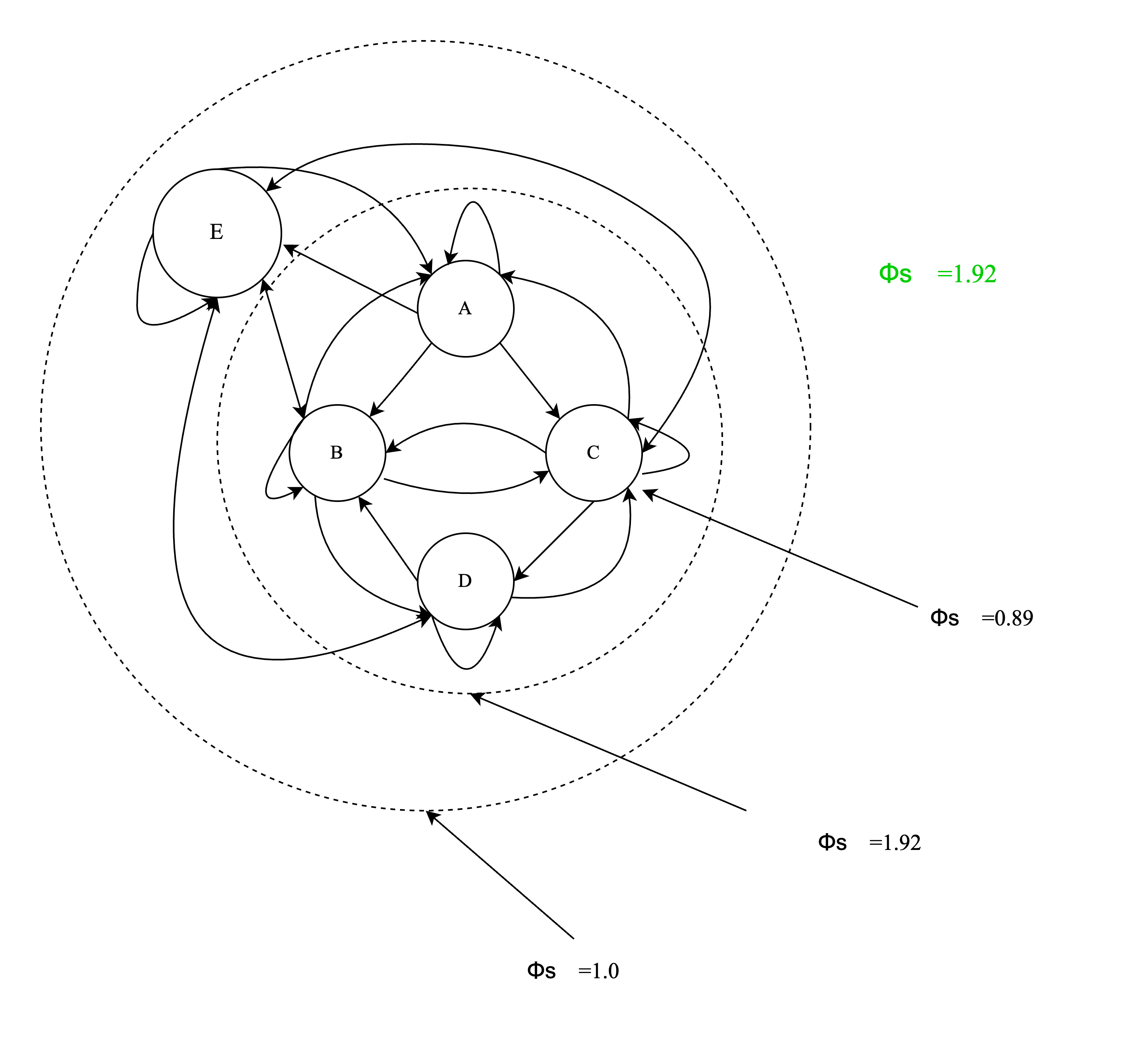
IIT begins from five phenomenological axioms — intrinsic existence, composition, information, integration and exclusion — and translates each into a postulate about what a physical substrate must be like to support experience.

The five axioms of IIT and their postulates — Figure 1. The five axioms of IIT and their translation into postulates on the physical substrate.

Intrinsic existence in system ABCD — Figure 2. *Intrinsic existence.* System ABCD has cause–effect power over itself.

Compositional structure — Figure 3. *Composition.* A mechanism built from input and output elements, combining into higher-order mechanisms.

Information: past and future states — Figure 4. *Information.* Each mechanism specifies a cause–effect repertoire over past and future states.

Exclusion postulate — Figure 5. *Exclusion.* Only the maximally irreducible structure exists: ABCD (Φ = 1.92) excludes ABCDE (Φ = 1.0) and C (Φ = 0.89).

2.2Φ and the minimum information partition

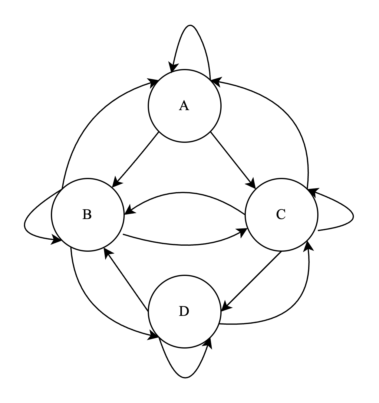
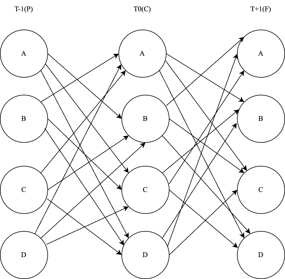
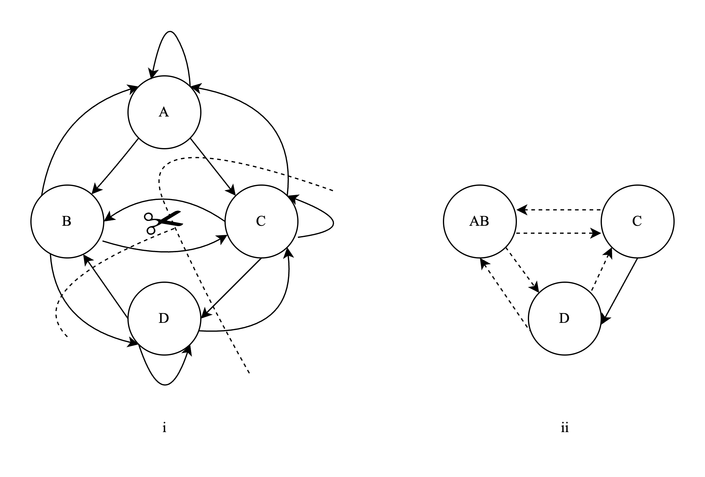
Φ measures how much of a system's cause–effect structure is lost when it is cut along its weakest link — the minimum information partition (MIP). A system with Φ > 0 is irreducible. A purely feedforward system, whose parts never mutually constrain one another's past and future, has Φ = 0.

Integration: partition into AB, C, D — Figure 6. *Integration.* Φ is computed by cutting the system (here into AB, C and D) and measuring how much cause–effect structure is lost at the weakest cut.

3Methods

3.1System pipeline

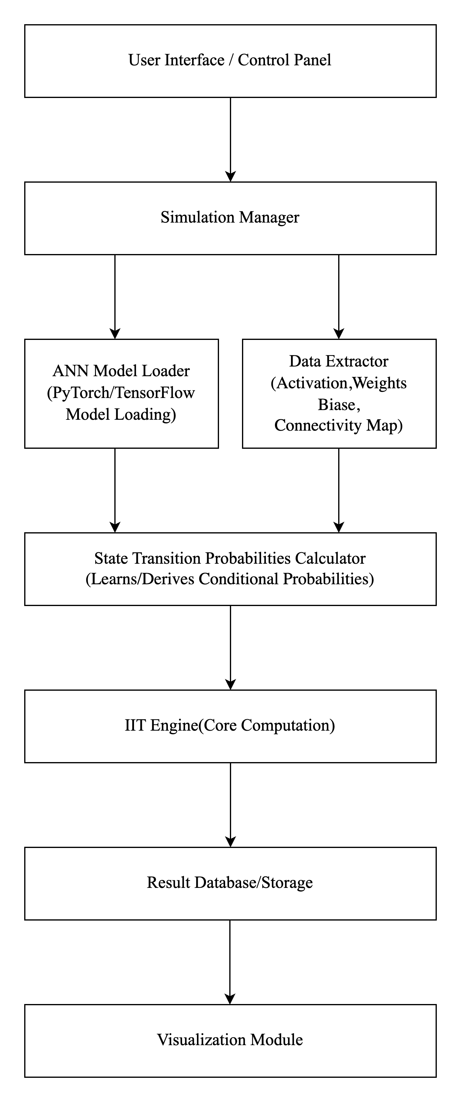
Networks are trained, internal states extracted, and integration quantified either exactly (Φ, small systems) or approximately (Φ*, scalable systems), followed by visualization and explainability analysis.

High-level system architecture — Figure 7. Model training → state extraction → TPM / covariance construction → Φ or Φ* computation → analysis. *(Click to enlarge.)*

3.2Exact Φ

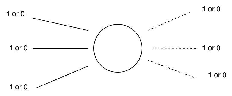
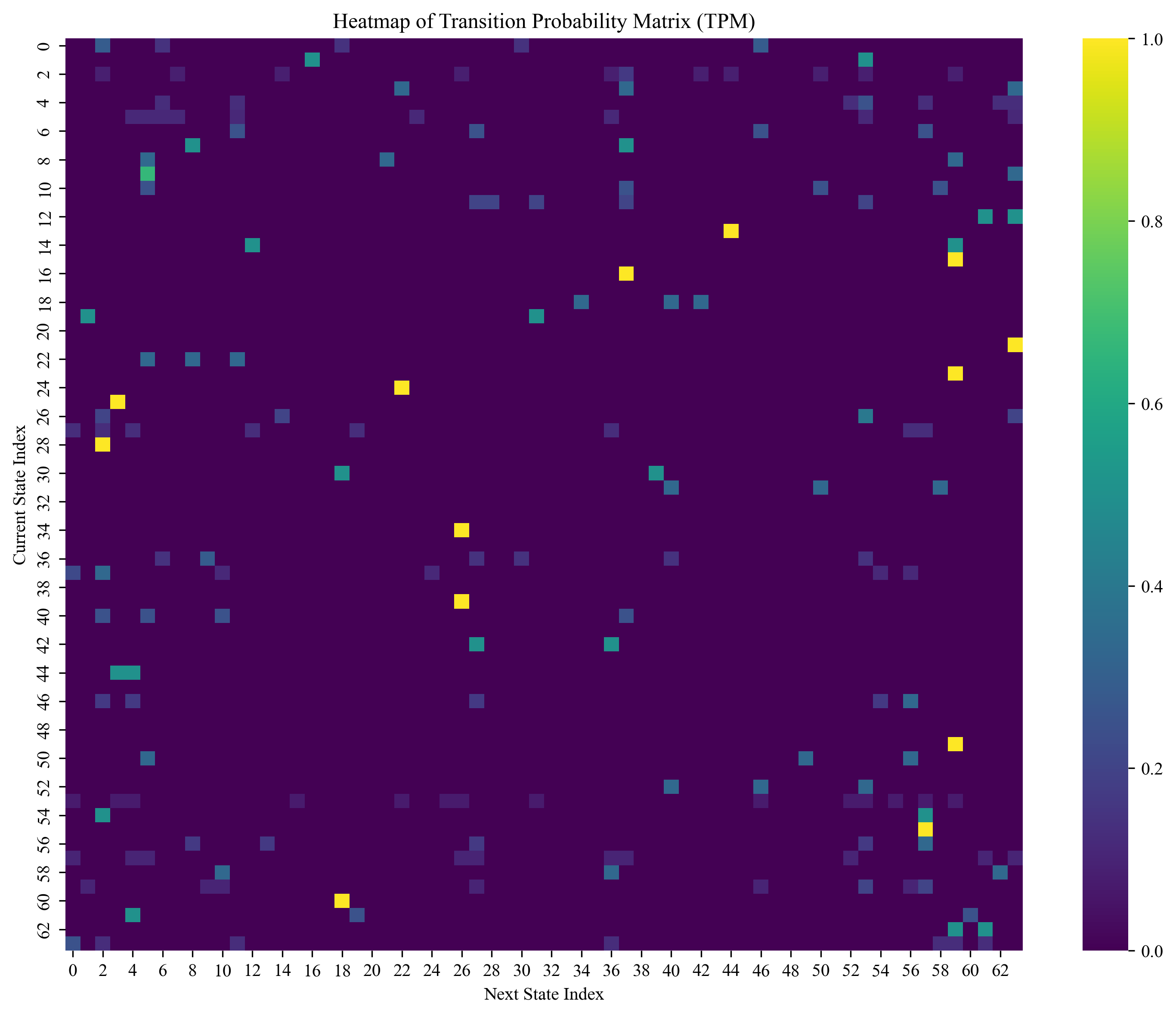
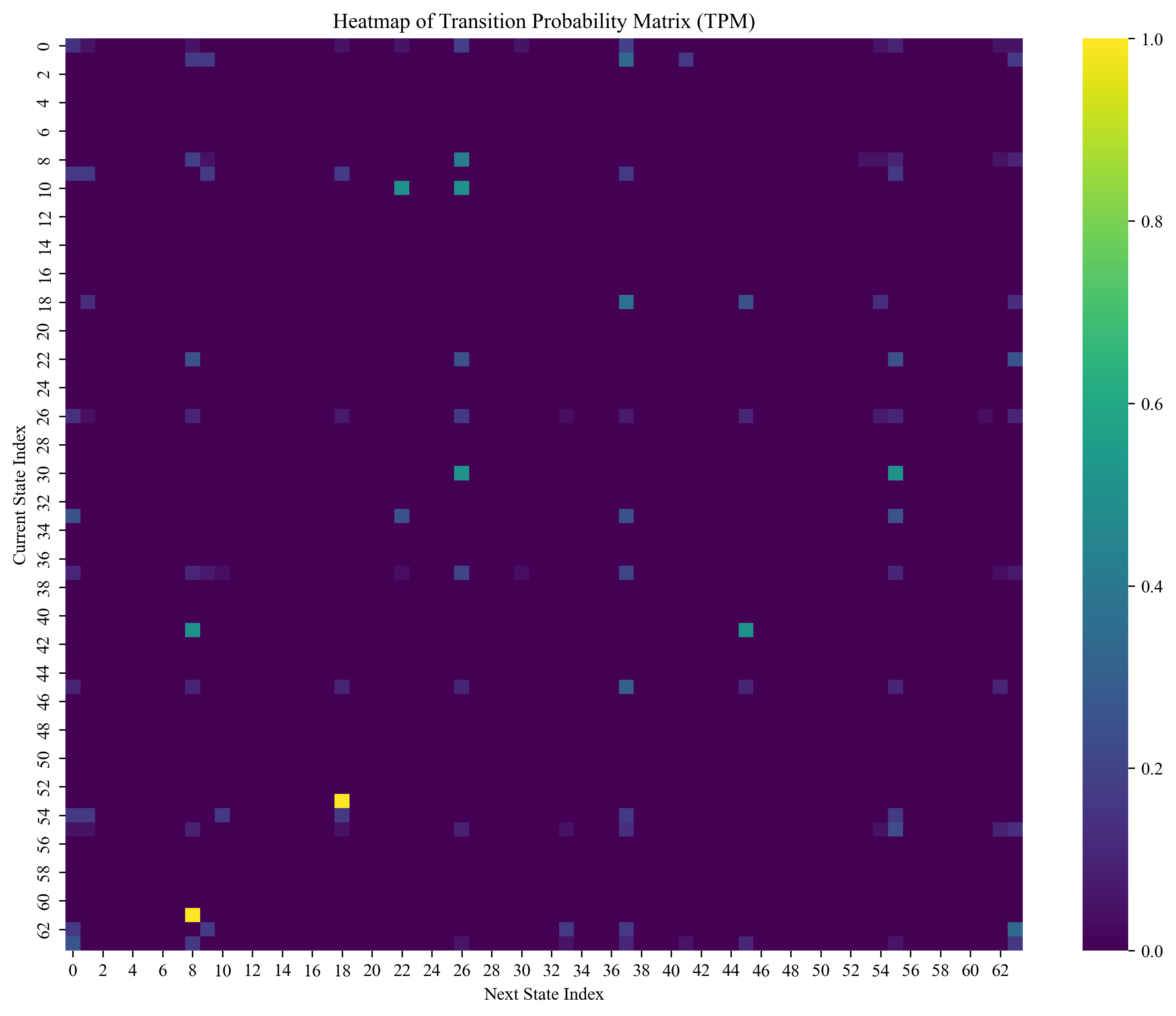
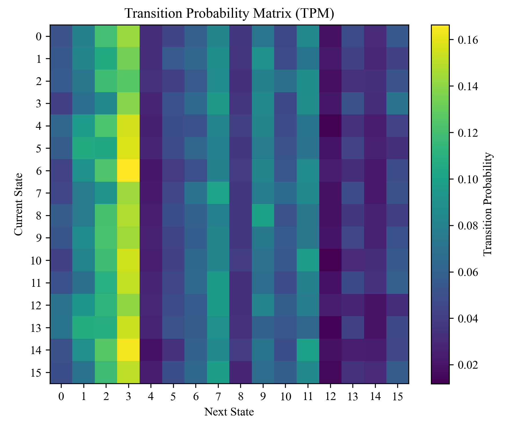
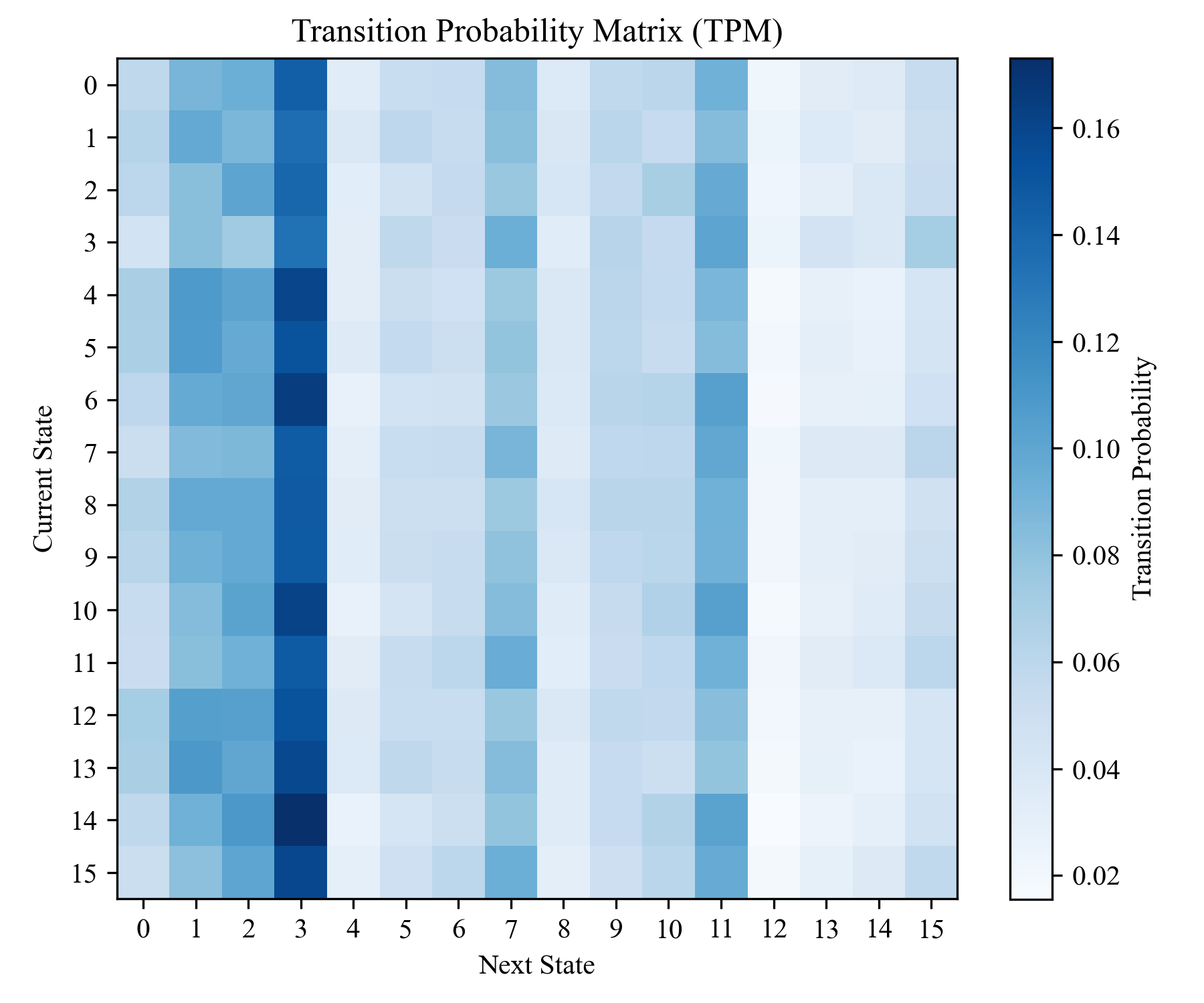
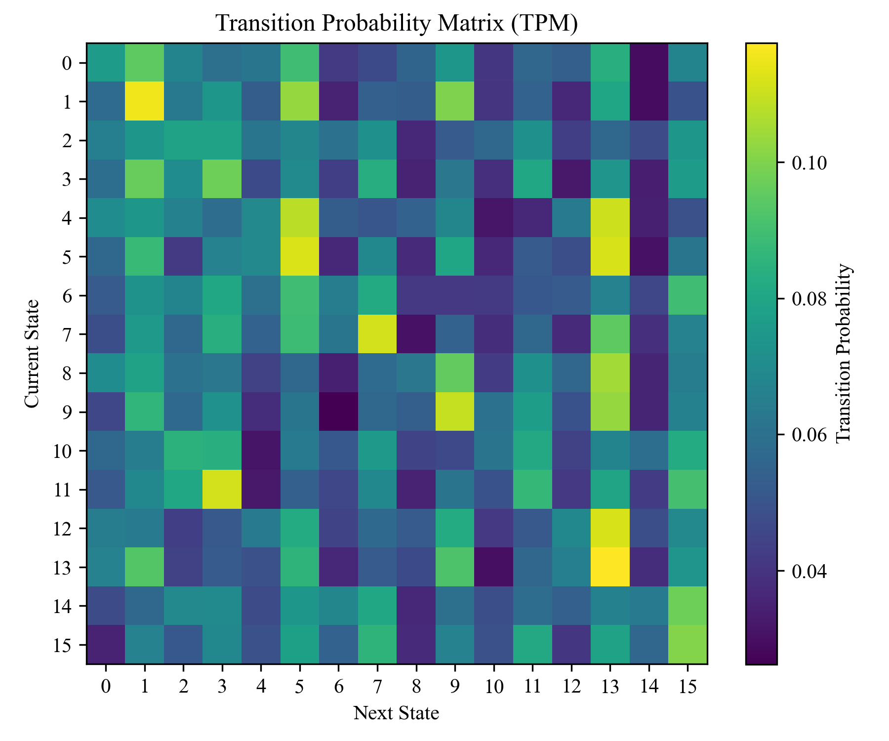
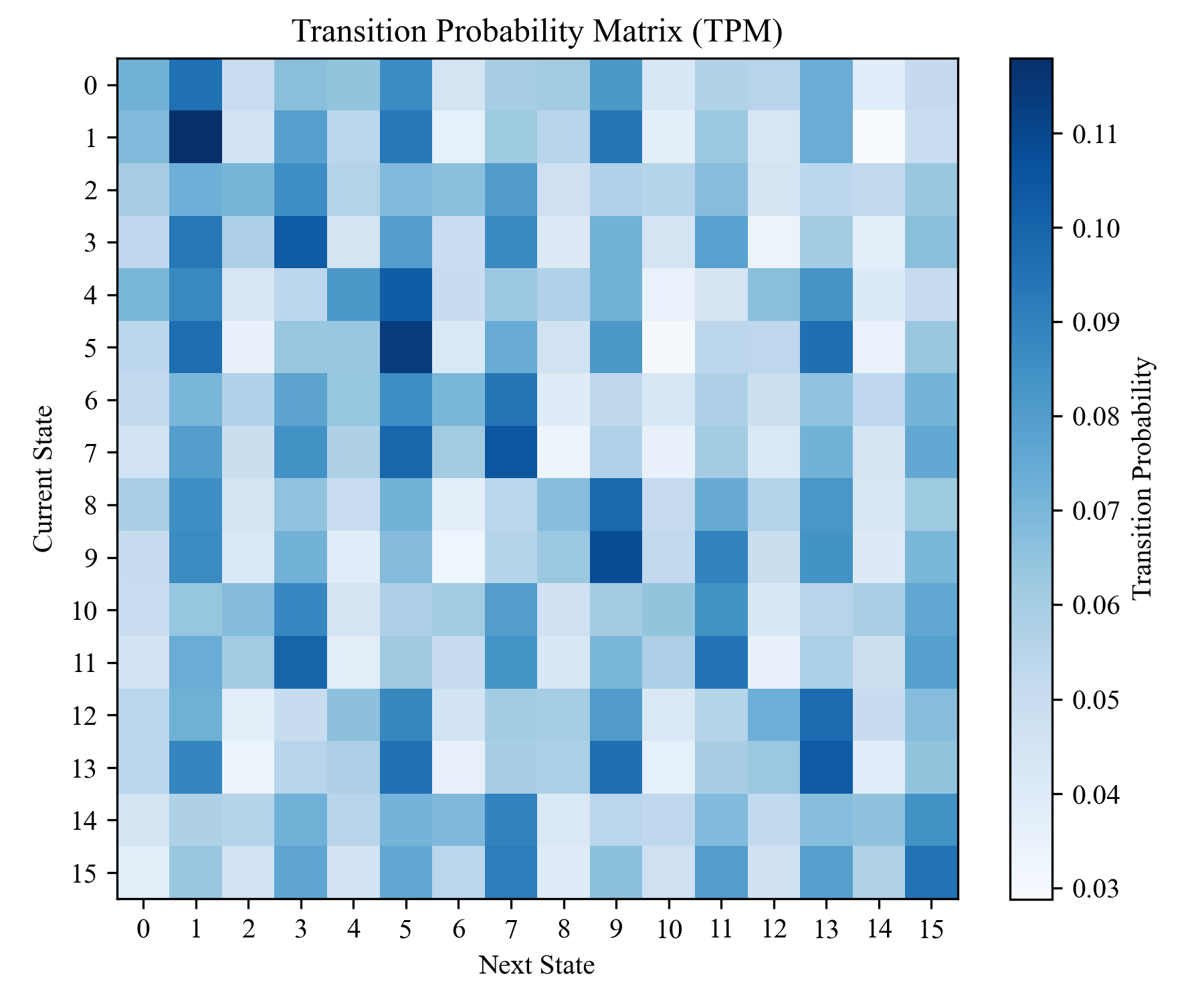
Small systems are modelled as discrete dynamical systems of binary nodes. Hidden activations are binarized (median threshold for feedforward layers, zero threshold for recurrent layers) and a transition probability matrix (TPM) of size 2ⁿ × 2ⁿ is estimated from observed state transitions. PyPhi then builds cause–effect repertoires, searches all bipartitions for the MIP, and returns the system-level Φ. The pipeline was validated on an XOR gate, which correctly returns Φ = 0.

3.3Approximate Φ*

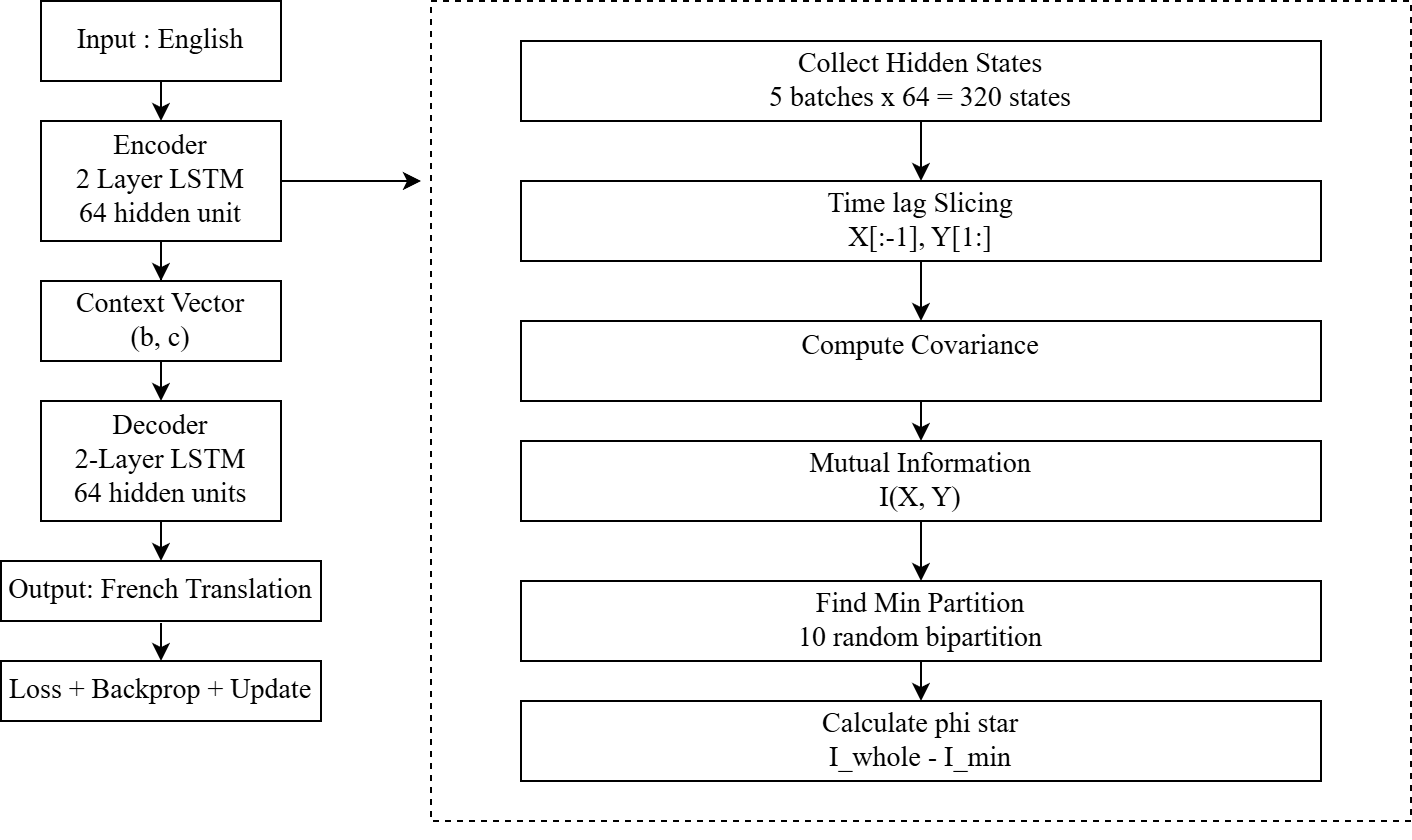
For larger networks, Φ* is estimated from hidden-state trajectories. With a lag τ, past and future blocks X and Y are formed, and under a Gaussian assumption the mutual information between two vector variables is

I(X;Y) = ½ · log₂ ( |Σ_X| · |Σ_Y| / |Σ_XY| )

For a bipartition into A and B, the information lost by the cut is φ = I(X;Y) − [I(X_A;Y_A) + I(X_B;Y_B)]. Φ* is the value of φ at the MIP.

3.4Φ versus Φ*

Table 1. The two measures answer different questions and must not be conflated.
	Exact Φ (IIT 3.0/4.0)	Approximate Φ*
Formal basis	Intrinsic cause–effect power over a TPM	Gaussian time-lagged mutual information
What it measures	Irreducibility of the cause–effect structure	Predictive information lost under a partition
Representation	Discrete binary states + TPM	Continuous hidden-state covariances
Partition search	All bipartitions, exact MIP (Earth Mover's Distance)	Sampled bipartitions, normalized MIB
Cost / scalability	`O(2ⁿ)`; ≲ 12 units	Polynomial (sampled); hundreds of units
Re: consciousness	Identified with consciousness by IIT	A proxy — not a consciousness measure
Reliability here	Exact but intractable at scale	Scalable but estimator-dependent

Idealized Phi vs epoch — Figure 8. Idealized Φ vs. epoch — expected to peak, then settle.

Idealized Phi-star vs epoch — Figure 9. Idealized Φ* vs. epoch — rises as internal representations form, then stabilizes.

4Feedforward networks: exact Φ

4.1Architectures

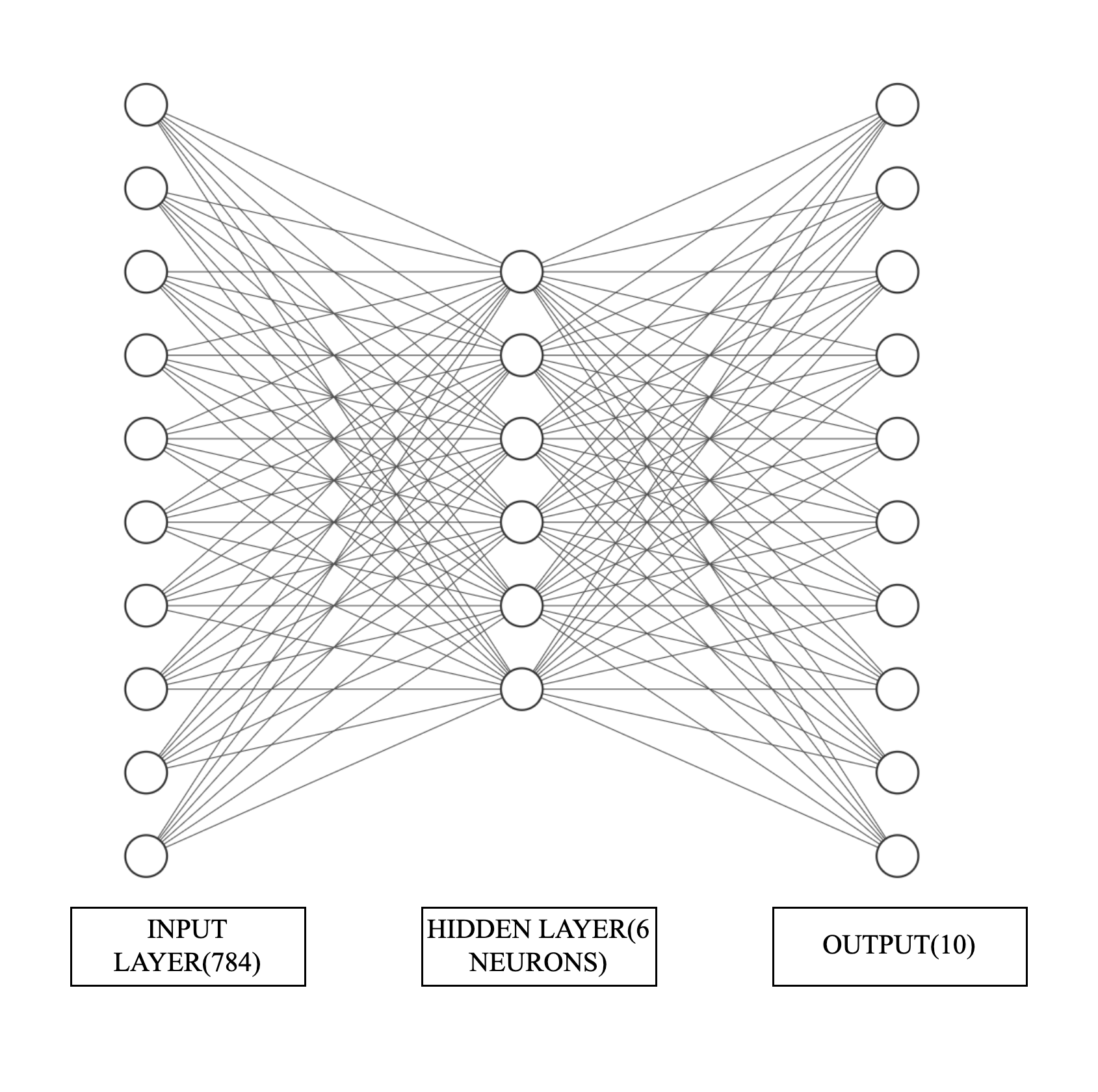
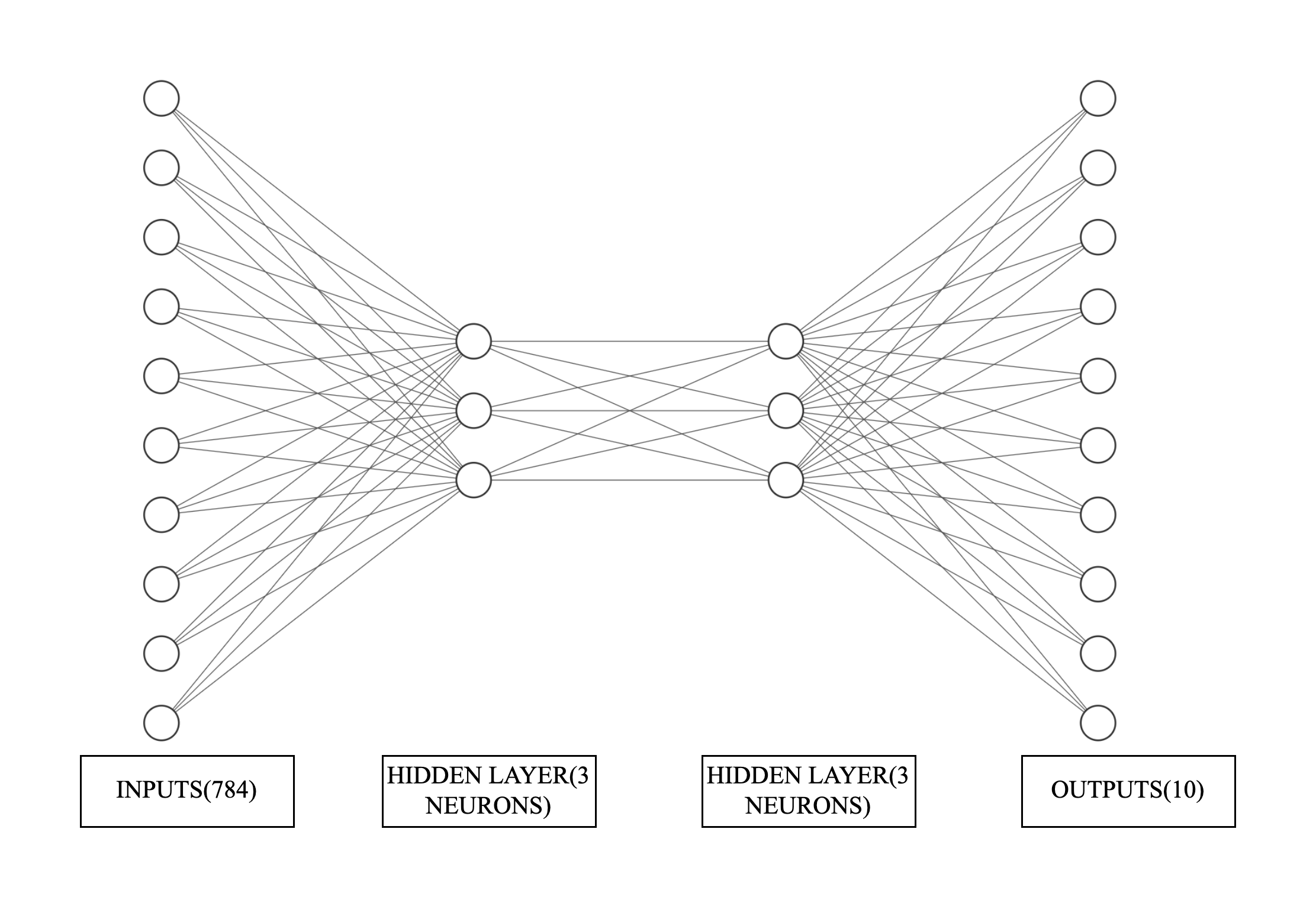
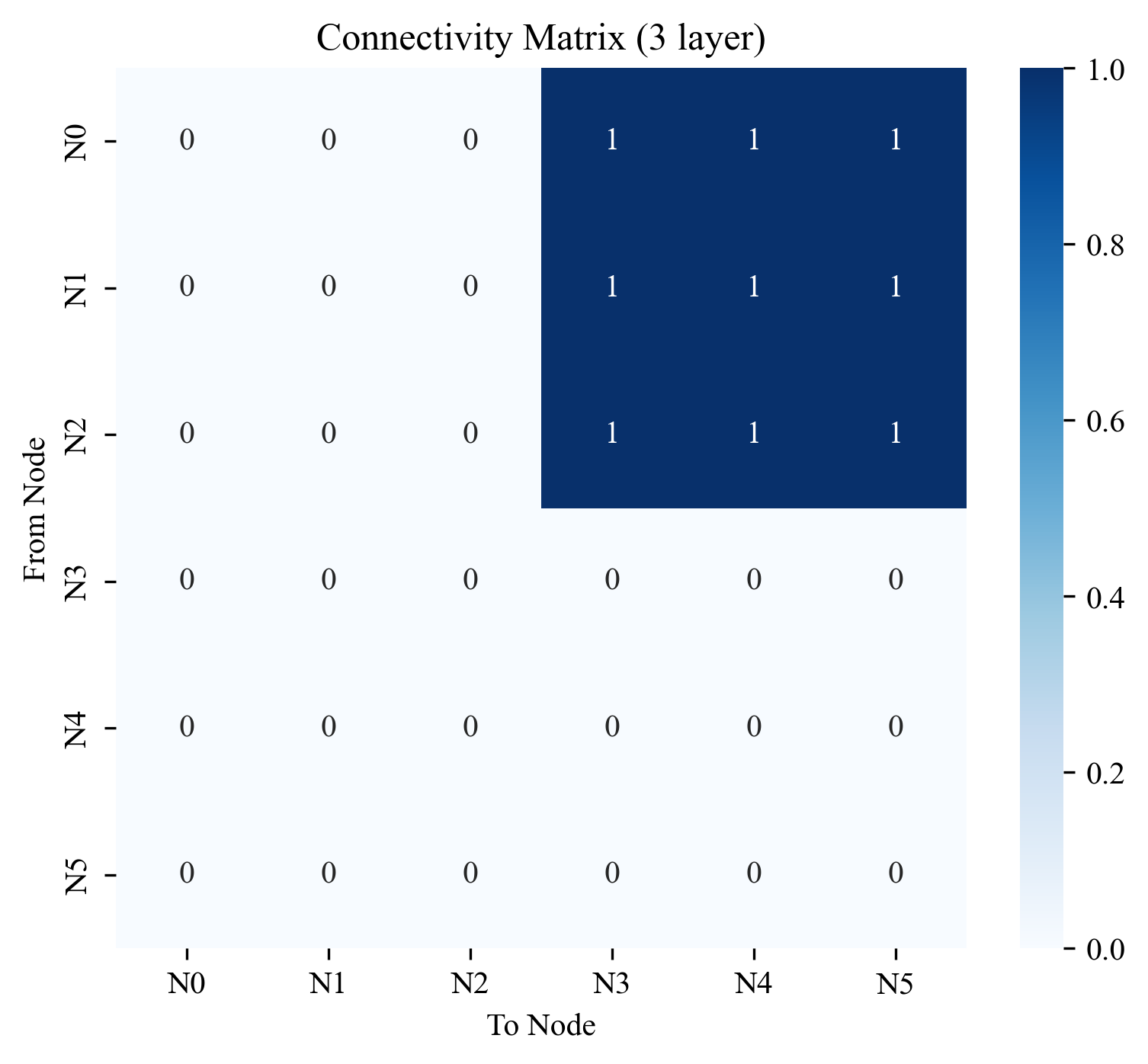
Two small MNIST classifiers keep exact Φ tractable: Architecture A (one hidden layer of six neurons) and Architecture B (two hidden layers of three neurons).

Feedforward Architecture A — Figure 10. Architecture A — one hidden layer, 6 neurons.

Feedforward Architecture B — Figure 11. Architecture B — two hidden layers, 3 neurons each.

Connectivity matrix Architecture A — Figure 12. Connectivity matrix, Architecture A.

Connectivity matrix Architecture B — Figure 13. Connectivity matrix, Architecture B — connections only between layers.

TPM heatmap Architecture A — Figure 14. TPM heatmap, Architecture A. Six neurons already require a 64 × 64 matrix — the root of the scaling problem.

TPM heatmap Architecture B — Figure 15. TPM heatmap, Architecture B.

4.2Result: Φ = 0

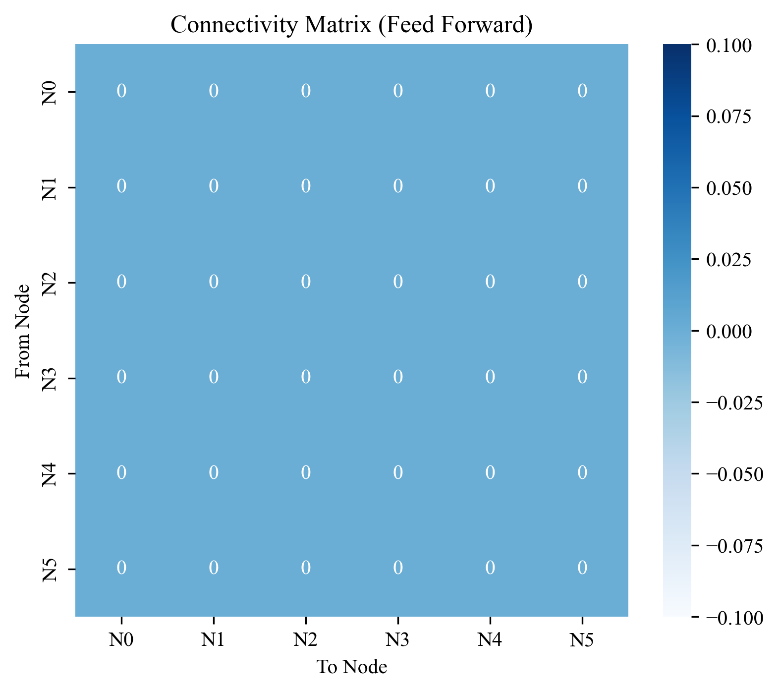
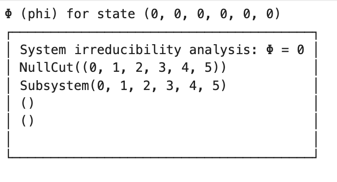
Both architectures return Φ = 0. With strictly unidirectional flow the hidden units never mutually constrain one another's past and future, so the system is fully reducible — even though it classifies digits accurately. Task competence and integrated information are already dissociated at the smallest scale.

Phi for architectures A and B — Figure 16. Φ for the default architectures A and B — both zero, as IIT predicts for purely feedforward systems.

4.3Rewiring: Φ = 2.47

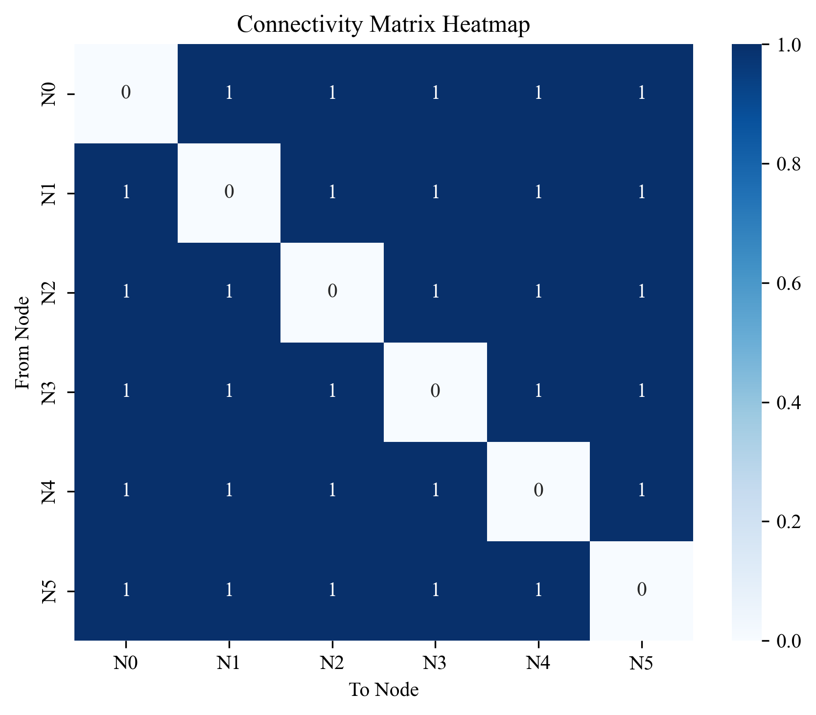
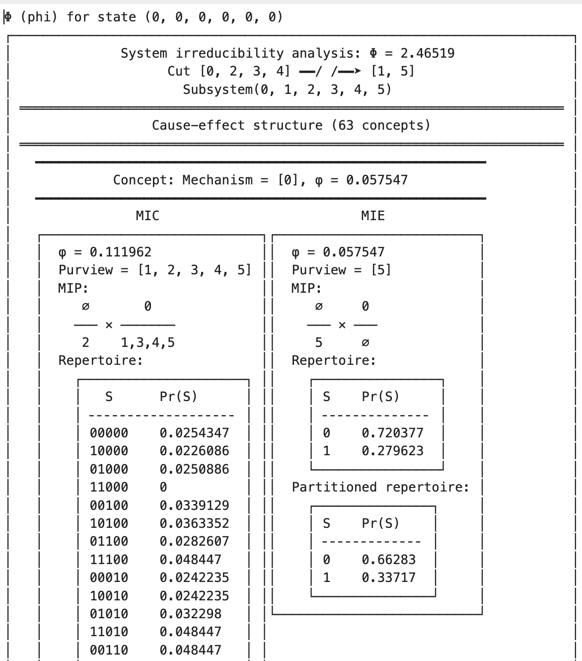
To show the difference is one of causal structure rather than function, we kept Architecture A and edited only its connectivity, replacing the feedforward graph with a densely recurrent one. Integrated information rose to Φ = 2.47 on the same task.

Modified recurrent connectivity — Figure 17. Rewired connectivity for Architecture A — recurrent, no self-loops.

Phi for modified connectivity — Figure 18. Φ = 2.47 after rewiring — the same computation, a different causal organization.

Interpretation. The rewired result is an illustrative manipulation of connectivity, not a property of the trained network. Its purpose is to isolate causal structure as the variable that moves Φ while the task is held fixed.

5Recurrent networks

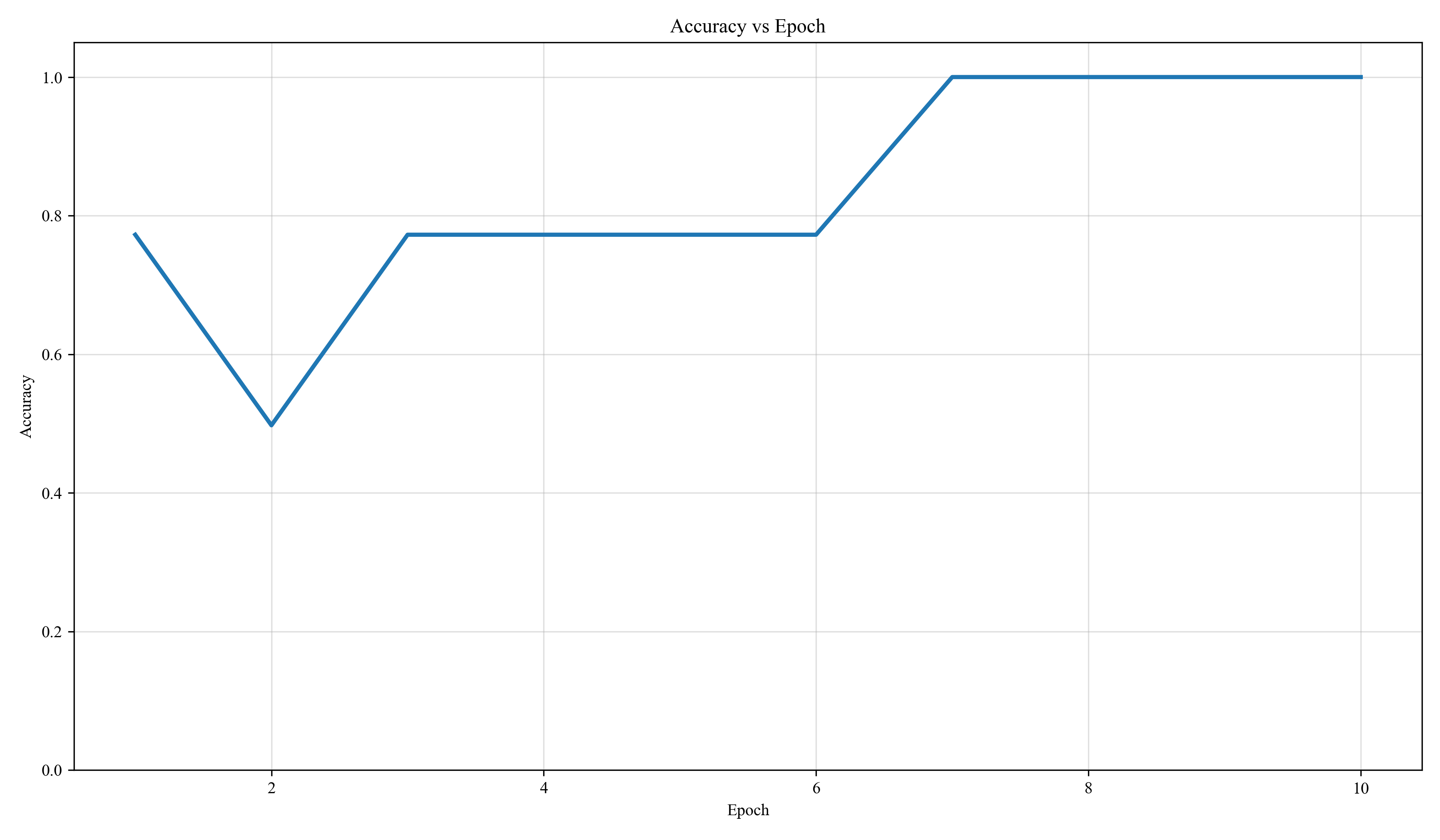
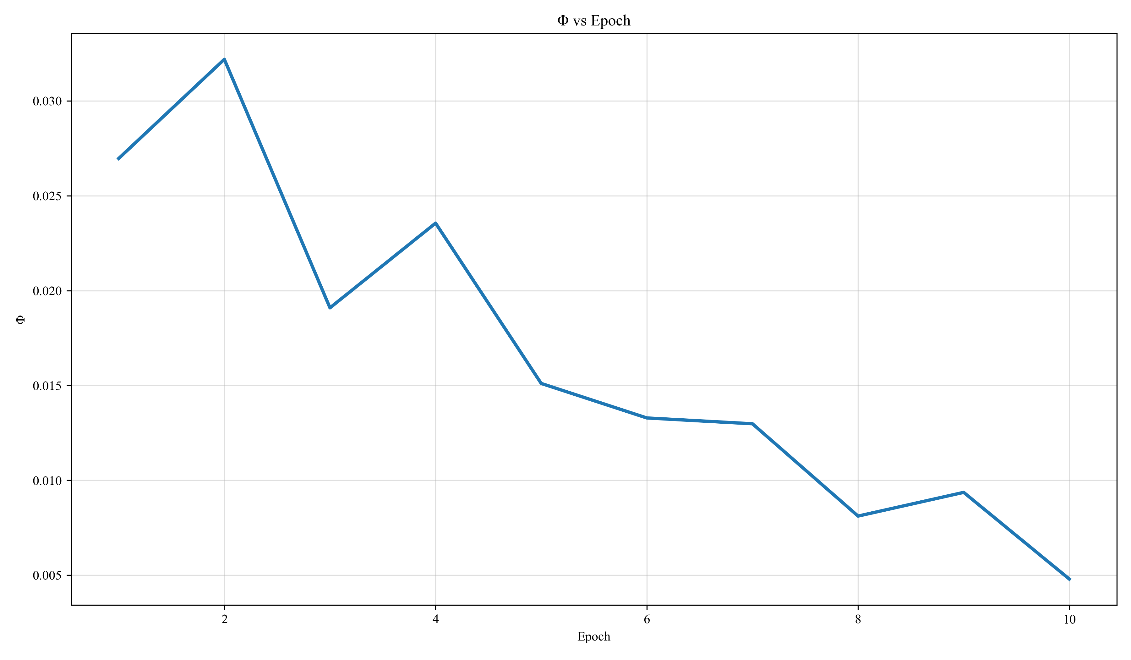
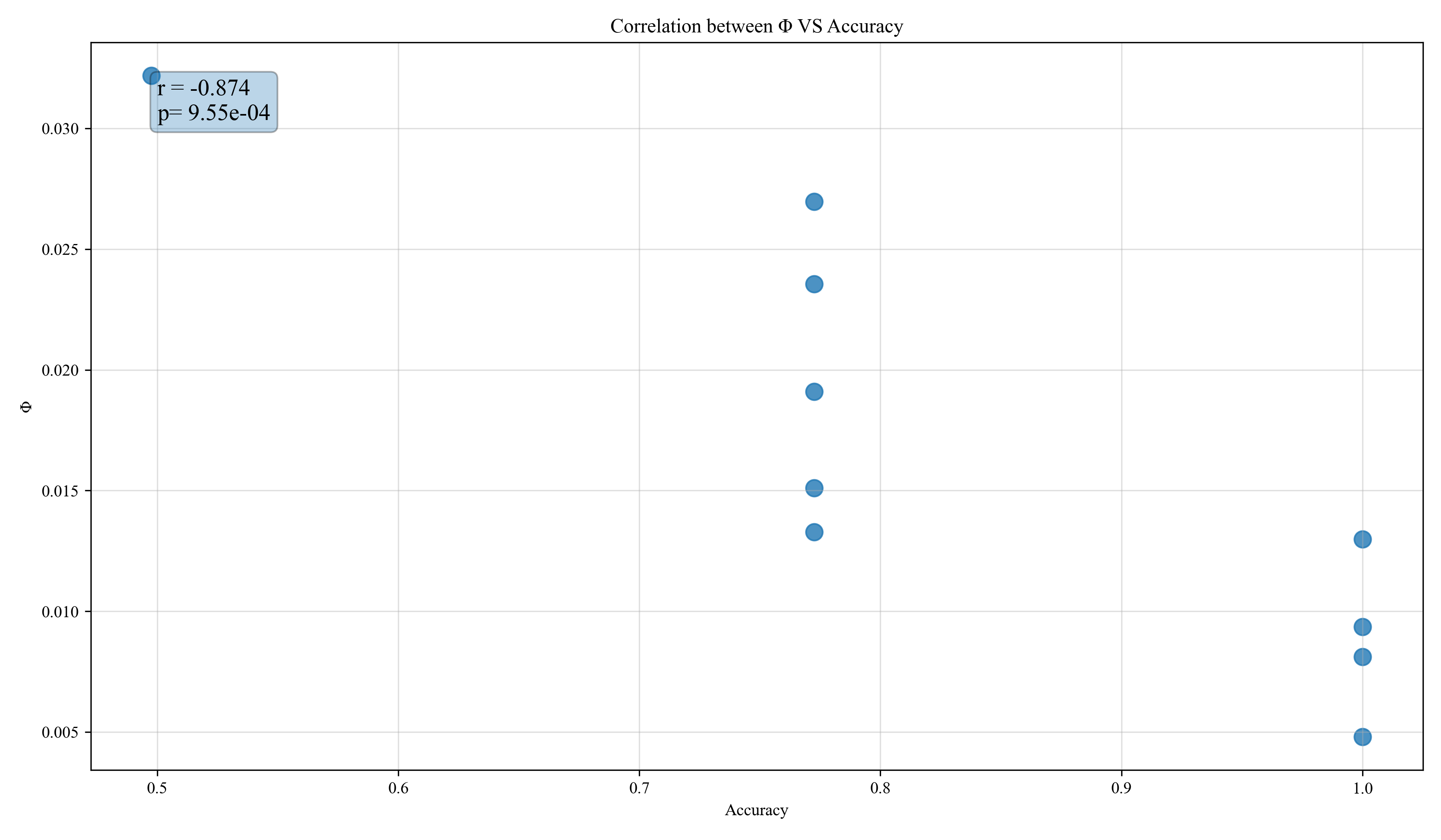
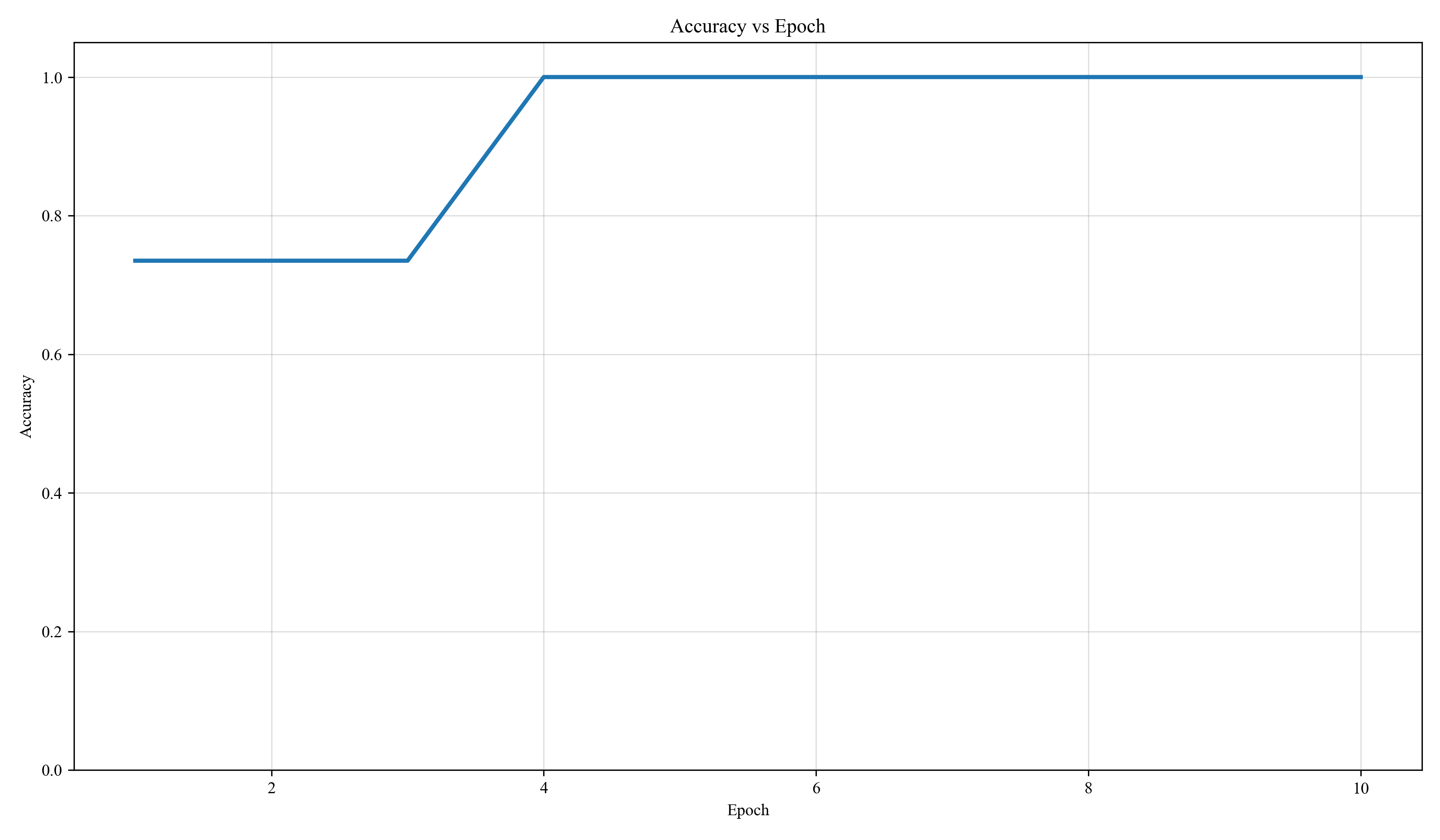
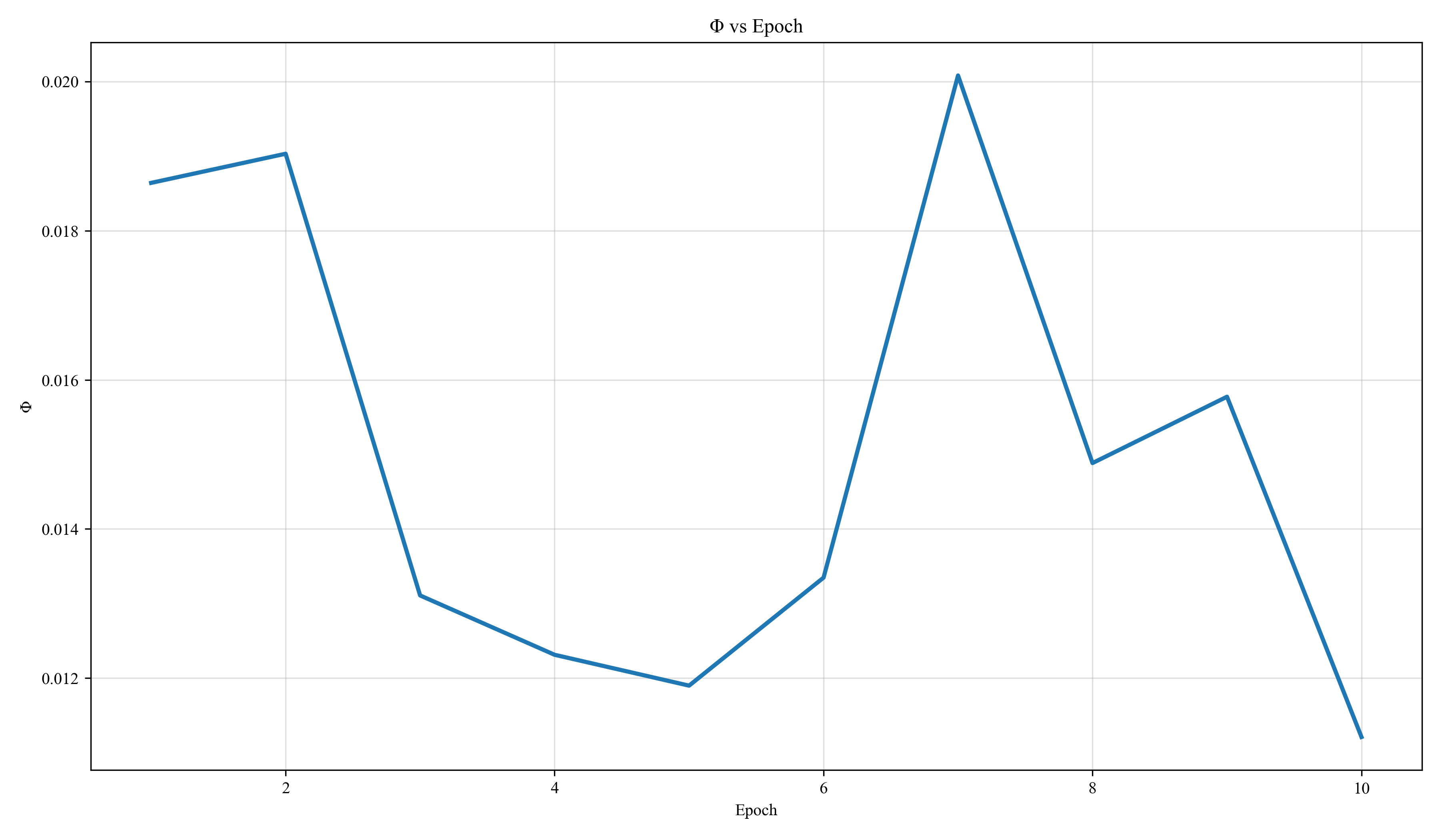
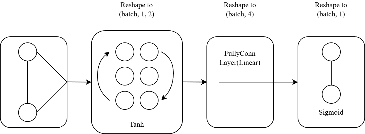
Because exact Φ costs O(2ⁿ), it is tractable only for tiny recurrent systems. We computed exact Φ for 4-unit RNN and GRU networks on a parity task, then moved to Φ* for 60-unit networks trained on a synthetic grammar-recognition task over the alphabet {X, Y, A, B, EOS}.

RNN architecture — Figure 19. Recurrent architecture used for the grammar task.

5.1Small systems (4 units)

RNN 4-unit original TPM — Figure 20. RNN (4 units) — original TPM.

RNN 4-unit MIP-cut TPM — Figure 21. RNN (4 units) — TPM after the MIP. The difference between these two matrices is what Φ quantifies.

GRU 4-unit original TPM — Figure 22. GRU (4 units) — original TPM.

GRU 4-unit MIP-cut TPM — Figure 23. GRU (4 units) — MIP-cut TPM.

RNN 4-unit accuracy — Figure 24. RNN (4) accuracy.

RNN 4-unit phi — Figure 25. RNN (4) Φ — declines as accuracy saturates.

RNN 4-unit phi-accuracy correlation — Figure 26. RNN (4) Φ–accuracy: better task performance coincided with *less* integration in this run.

GRU 4-unit accuracy — Figure 27. GRU (4) accuracy — saturates early.

GRU 4-unit phi — Figure 28. GRU (4) Φ — non-monotonic.

5.2Scalable systems (60 units)

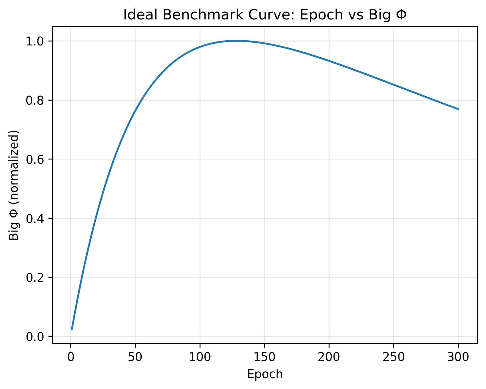
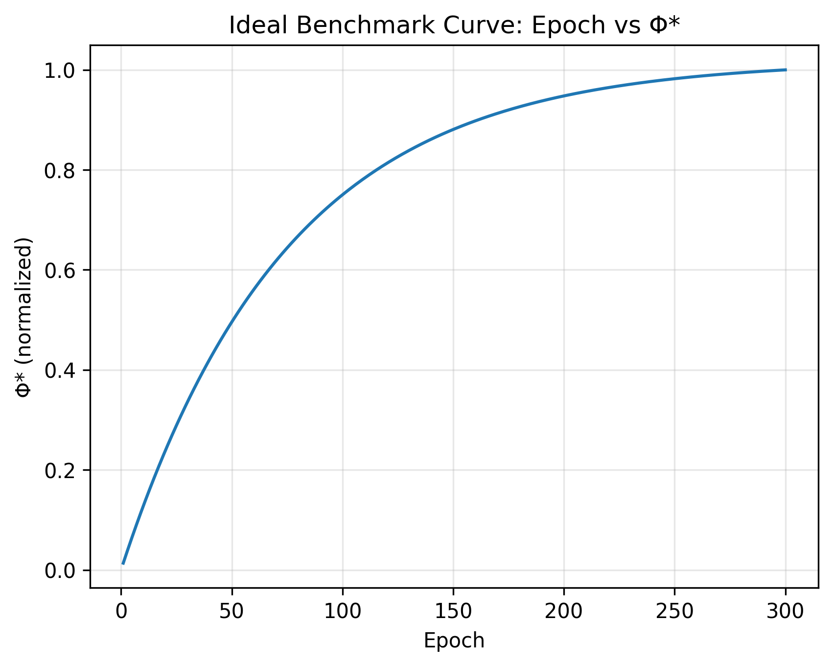
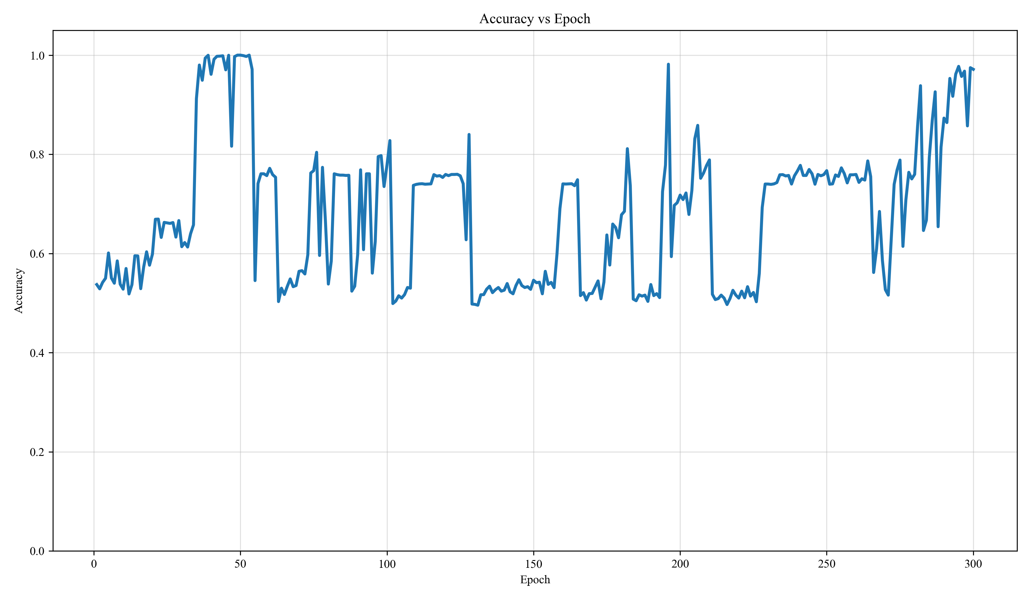
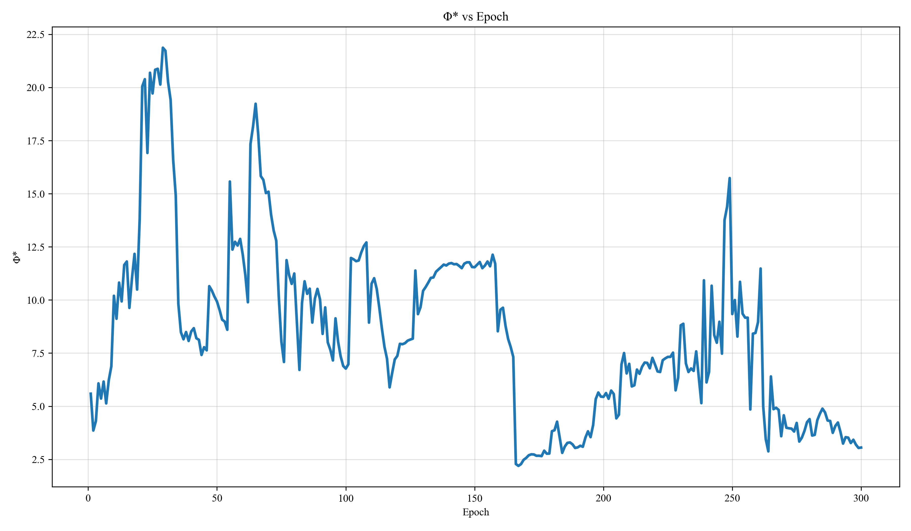
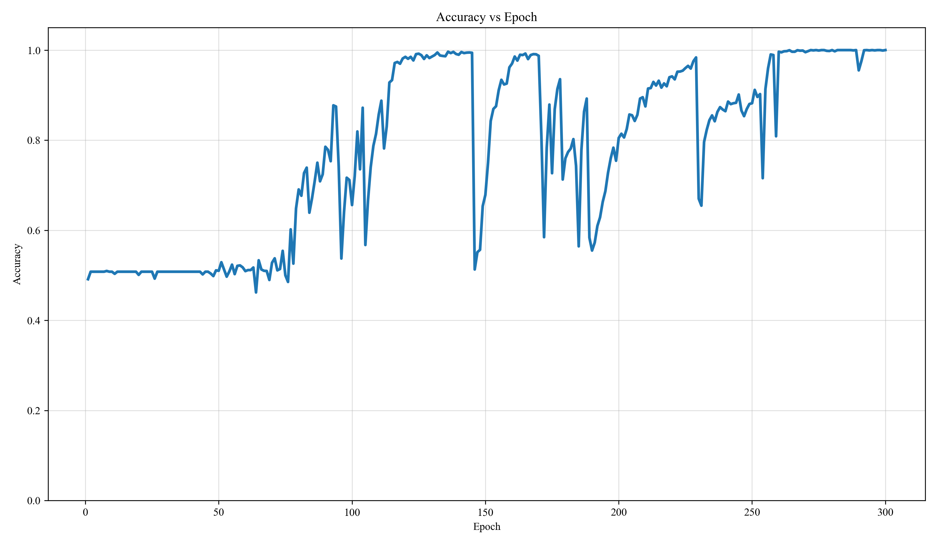
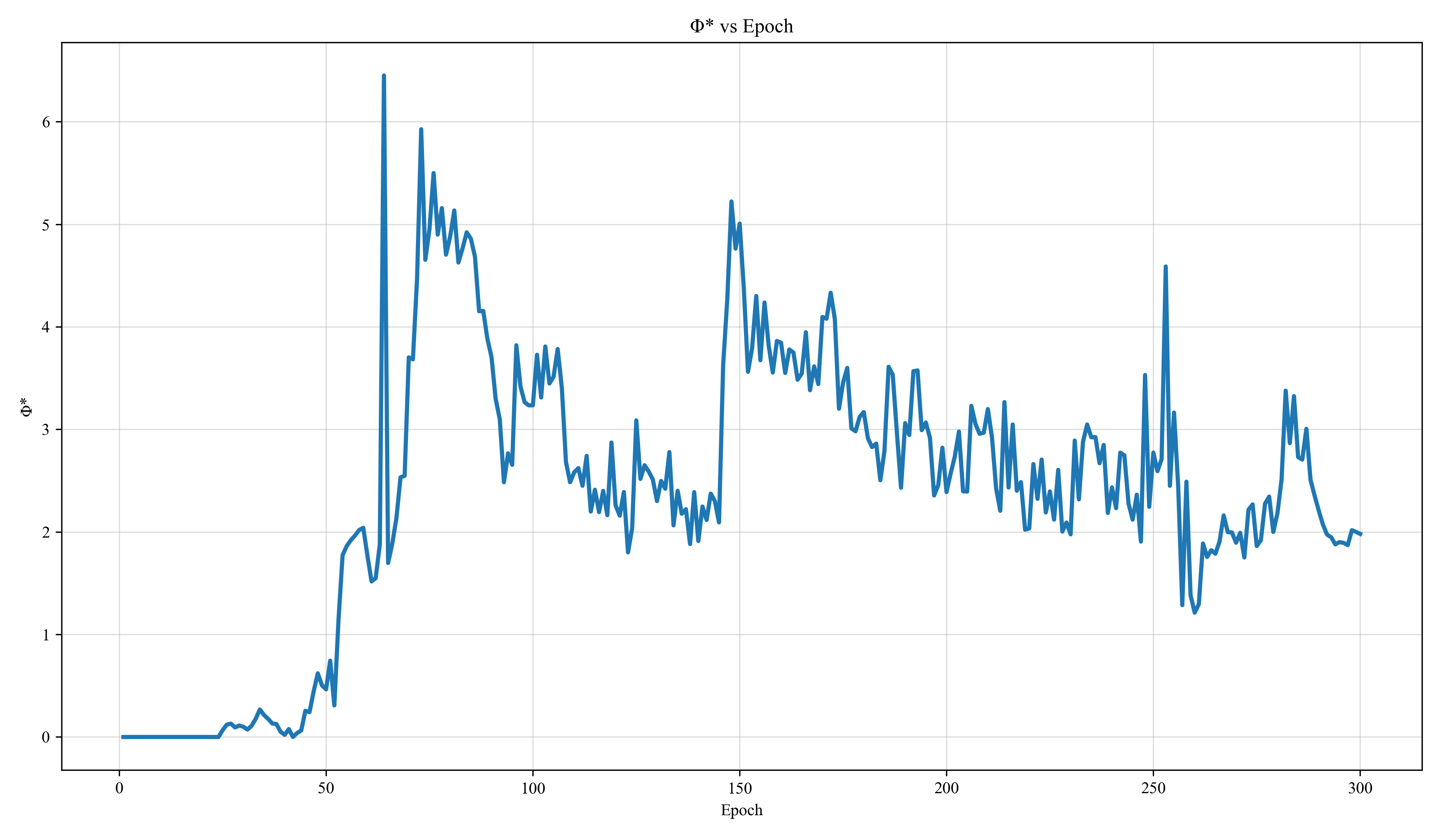
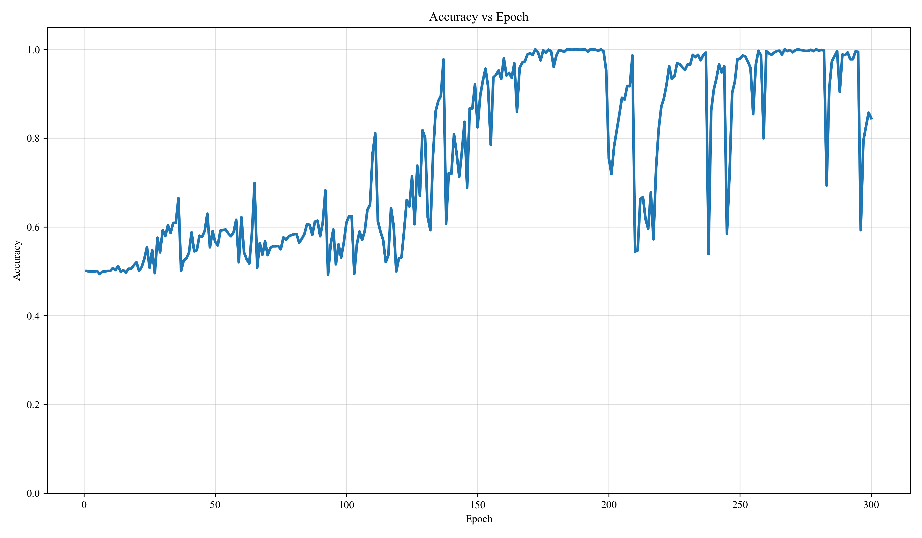
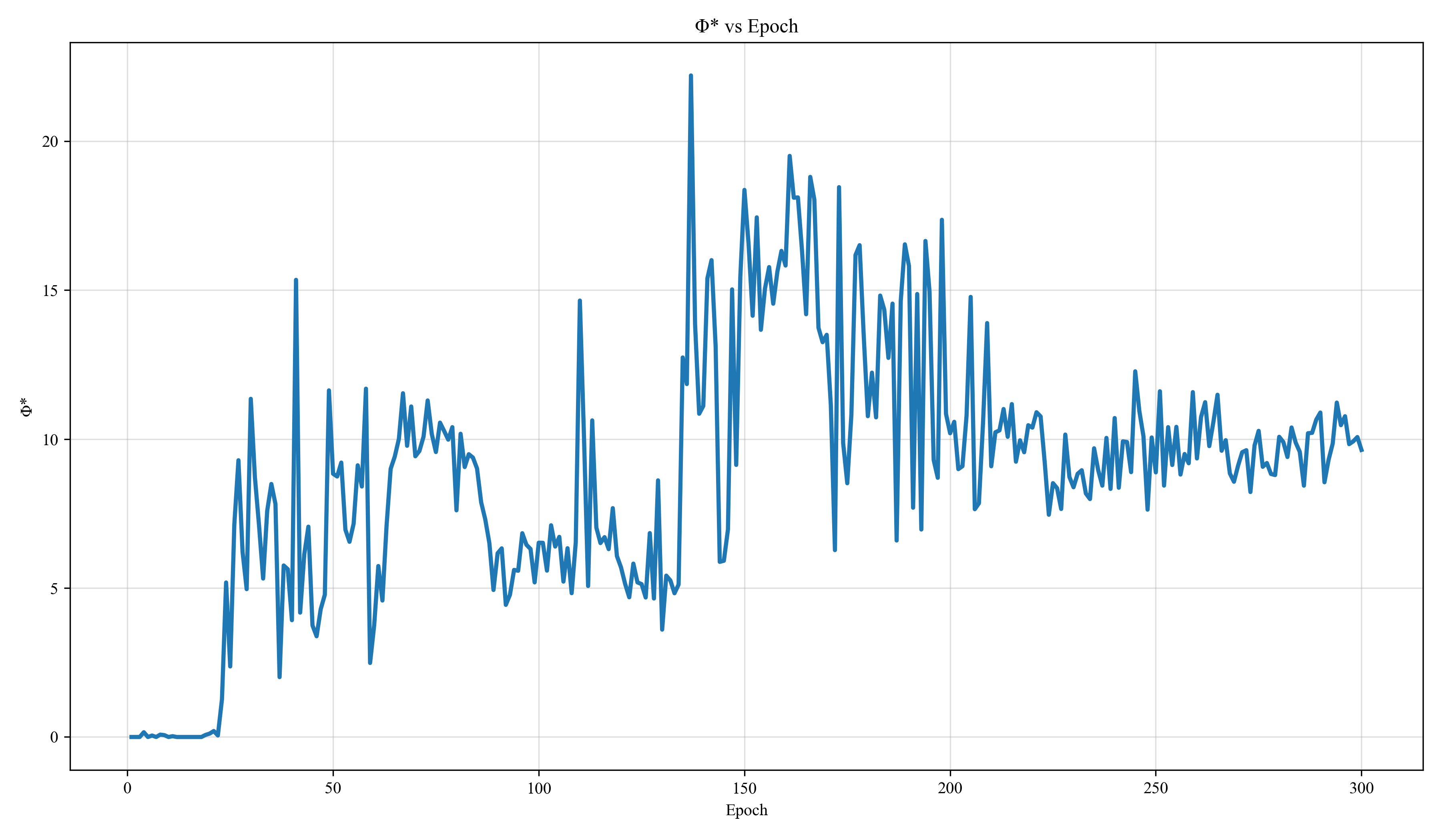
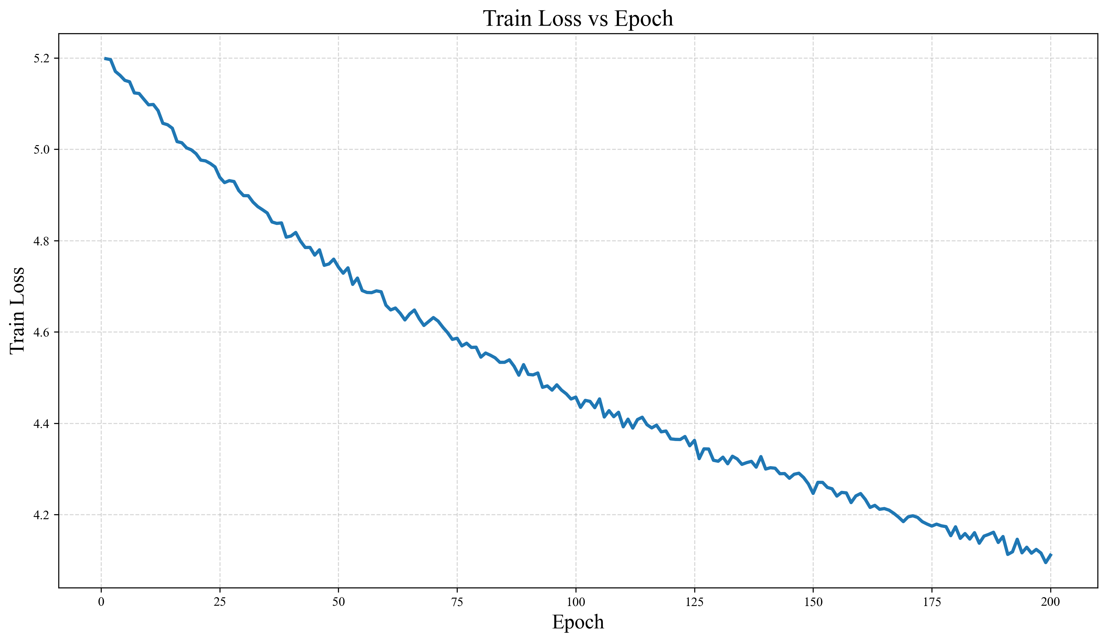
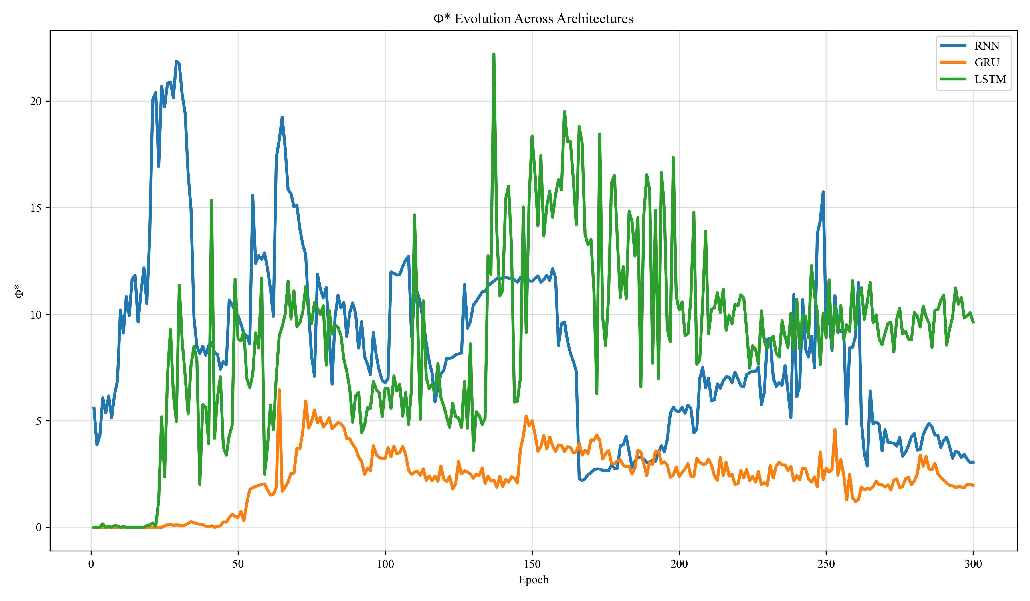
These were the first Φ* results, obtained while establishing that Gaussian Φ* could be tracked during training. They are shown for completeness and for contrast with the matched estimator in section 6.

RNN 60 accuracy — Figure 29. RNN (60) accuracy.

RNN 60 phi-star — Figure 30. RNN (60) Φ*.

RNN 60 correlation — Figure 31. RNN (60) Φ*–accuracy.

GRU 60 accuracy — Figure 32. GRU (60) accuracy.

GRU 60 phi-star — Figure 33. GRU (60) Φ*.

GRU 60 correlation — Figure 34. GRU (60) Φ*–accuracy.

LSTM 60 accuracy — Figure 35. LSTM (60) accuracy.

LSTM 60 phi-star — Figure 36. LSTM (60) Φ*.

LSTM 60 correlation — Figure 37. LSTM (60) Φ*–accuracy.

5.3Sequence-to-sequence LSTM

Seq2seq architecture — Figure 38. LSTM encoder–decoder (128-d embeddings, 64-d hidden, dropout 0.3).

Architecture with phi tracking — Figure 39. Φ* tracking — encoder hidden states are collected during training as a multivariate time series.

LSTM advance phi vs epoch — Figure 40. Φ* vs. epoch (translation): rises from ≈0.3 to ≈5.5 bits, then plateaus.

LSTM advance training loss — Figure 41. Training loss. Higher integration accompanied lower loss in this run (r ≈ −0.89).

5.4Initial cross-architecture comparison

6Matched estimation pipeline

6.1Limitations addressed

The initial implementation was designed to demonstrate the feasibility of computing Gaussian Φ* during training. Before drawing quantitative cross-architecture conclusions, we re-examined the estimation pipeline and identified three methodological limitations that introduce systematic bias into such comparisons:

Unmatched settings. Architectures were scored with different numbers of hidden-state samples (2000 for GRU vs. 500 for RNN and LSTM). Gaussian mutual information depends on how well the covariance is estimated.
Numerical instability. Hidden-state trajectories are strongly correlated and low-rank, so the raw sample covariance is near-singular. The initial estimator produced mutual information of tens to hundreds of bits — unrealistically large for the scale of the recorded dynamics, and indicative of numerical ill-conditioning rather than genuine information content.
Single-run evaluation. Each architecture came from a single unseeded training run, so correlations carried no error bars.

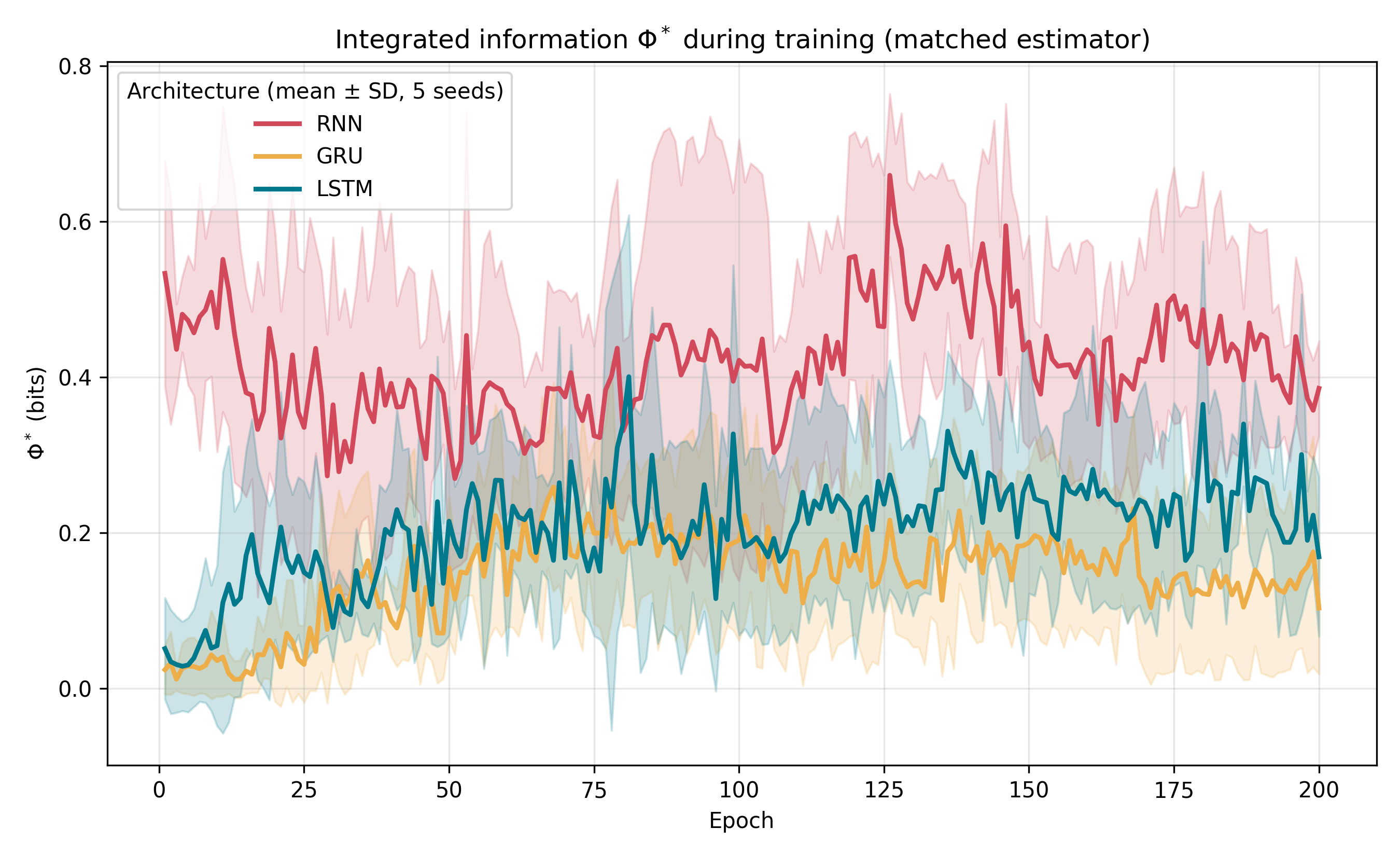
The refined pipeline uses one shared estimator for every architecture, with per-variable standardization and diagonal covariance shrinkage (bounding the log-determinant), and five independent training runs per architecture with different random seeds — quantifying the variability introduced by stochastic weight initialization and optimization. Whole-system information now falls to a sensible 14–17 bits.

6.2Results

Matched multi-seed phi-star during training — Figure 43. Matched, five-seed Φ* during training (mean ± SD bands). The RNN sustains the highest Φ*; GRU and LSTM overlap at lower values — **reversing the initial ordering**.

Matched multi-seed accuracy — Figure 44. Accuracy for the matched runs (mean ± SD). All architectures approach ceiling accuracy despite differing threefold in Φ*.

Phi-star versus accuracy — Figure 45. Φ* vs. accuracy, pooled over five seeds. Correlations are weak with per-seed error bars spanning zero — **integration and task performance are dissociated**.

Table 2. Matched, five-seed results (mean ± SD across seeds).
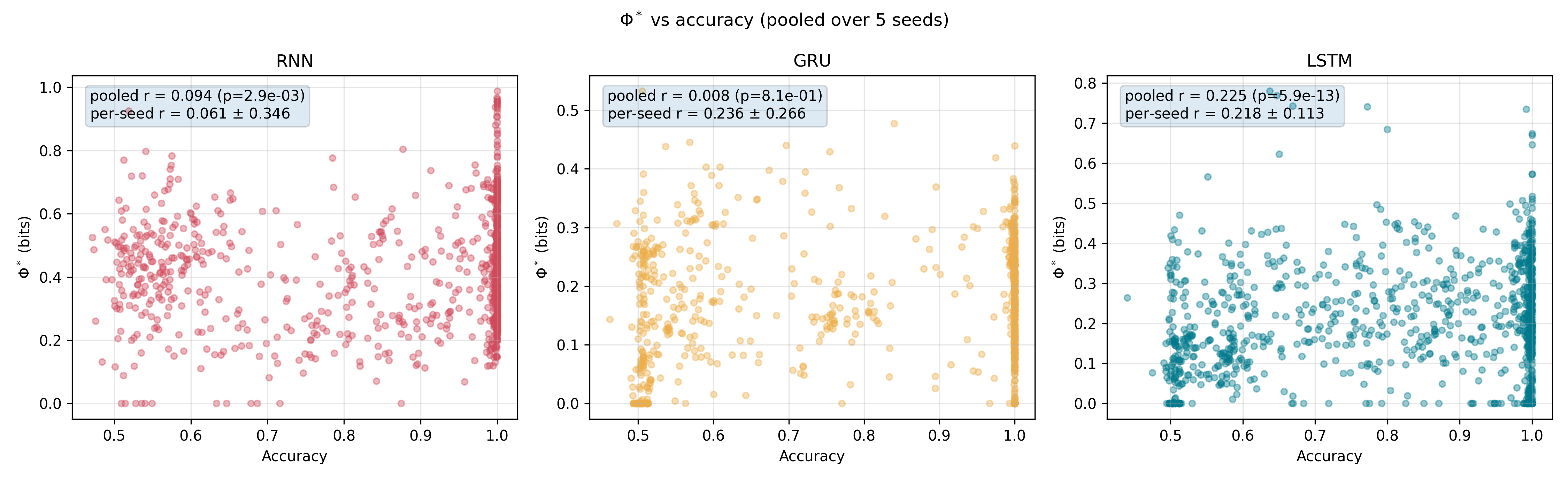
Architecture	Mean Φ*	Final accuracy	Φ*–accuracy r	Initial impl. (contrast)
RNN (60)	0.42 ± 0.07	1.00 ± 0.00	0.06 ± 0.35	8.51 (ranked 2nd)
GRU (60)	0.15 ± 0.07	1.00 ± 0.00	0.24 ± 0.27	2.39 (ranked 3rd)
LSTM (60)	0.21 ± 0.03	0.93 ± 0.10	0.22 ± 0.11	8.88 (ranked 1st)

7Validity and sensitivity

7.1Synthetic validation

Because the matched pipeline yields much smaller Φ* values than the initial one, it is essential to ask whether Φ* measures genuine integration. We tested the estimator on synthetic linear dynamical systems with known structure: two 5-dimensional blocks that either evolve independently or are coupled.

Table 3. Φ* on synthetic systems (mean ± SD over 5 seeds). Φ* rises with genuine coupling but has a non-zero floor.
Coupling	0.00	0.10	0.15	0.20	0.30
Φ*	0.087 ± 0.006	0.062 ± 0.008	0.105 ± 0.013	0.207 ± 0.016	0.375 ± 0.019

Φ* does increase with genuine coupling, confirming real sensitivity. But it also has a non-zero floor of ≈0.09 for a truly independent system — reflecting the known tendency of Gaussian Φ estimators to conflate integration with redundancy. Only differences well above this floor are meaningful.

7.2Estimator sensitivity

Sensitivity of phi-star to estimator settings — Figure 46. Sensitivity of Gaussian Φ* to estimator settings on a fixed trained-LSTM trajectory. *Left:* Φ* stabilizes only above ~1000 samples. *Centre:* Φ* reads zero at 20 sampled bipartitions (the initial setting) and stabilizes only at ≥100. *Right:* Φ* swings from 0.51 to 0.10 as shrinkage varies.

The methodological result. Rather than showing that one recurrent architecture is intrinsically more integrated than another, these results show that current scalable estimators remain highly sensitive to methodological choices — an observation that is itself an important result for future empirical studies applying IIT to artificial neural networks.

8Φ* and SHAP

SHAP measures external feature importance; Φ* probes internal integration. We correlated epoch-wise Φ* with the magnitude of Gradient-SHAP attributions.

Phi-star vs SHAP, RNN — Figure 47. RNN — weak negative association (r = −0.27).

Phi-star vs SHAP, LSTM — Figure 48. LSTM — weak positive association (r = 0.36).

Phi-star vs SHAP, GRU — Figure 49. GRU — weak negative association; log–log axes reveal a nonlinear decay.

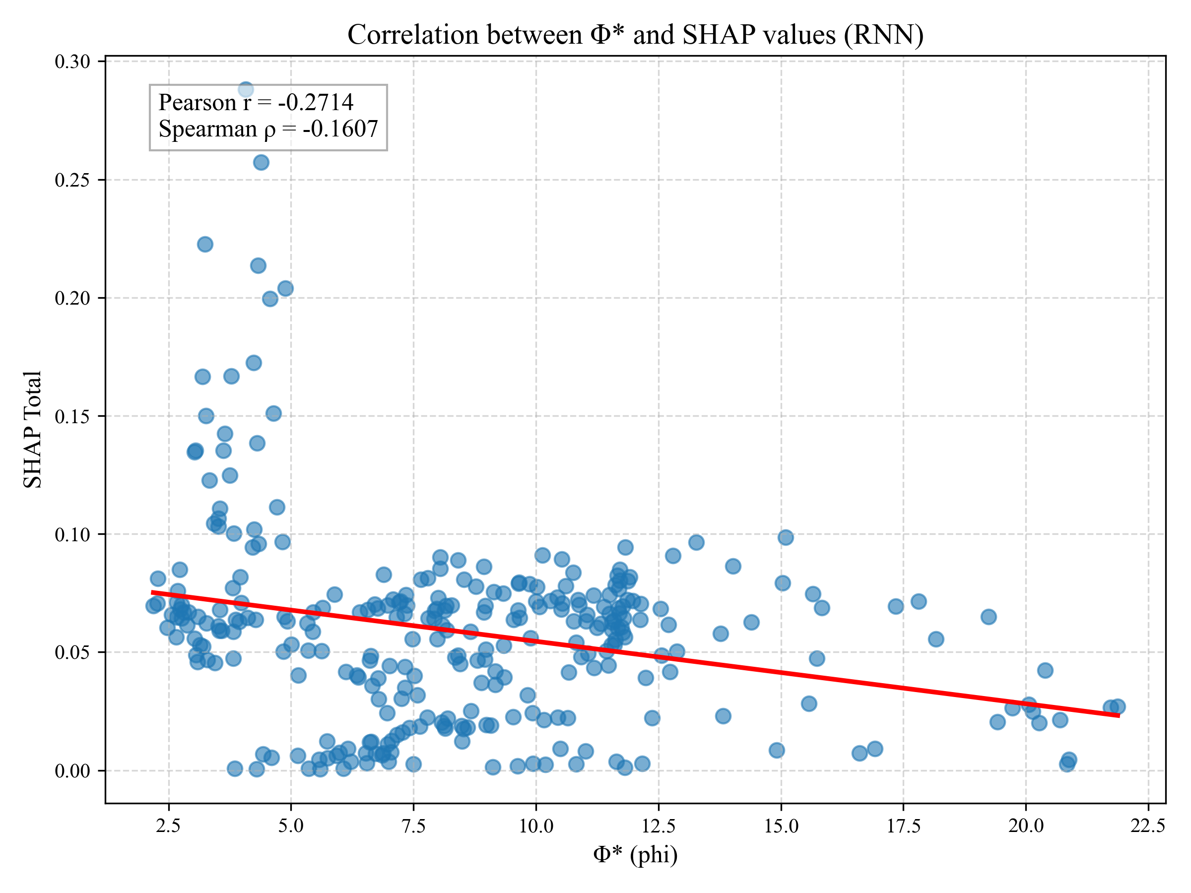
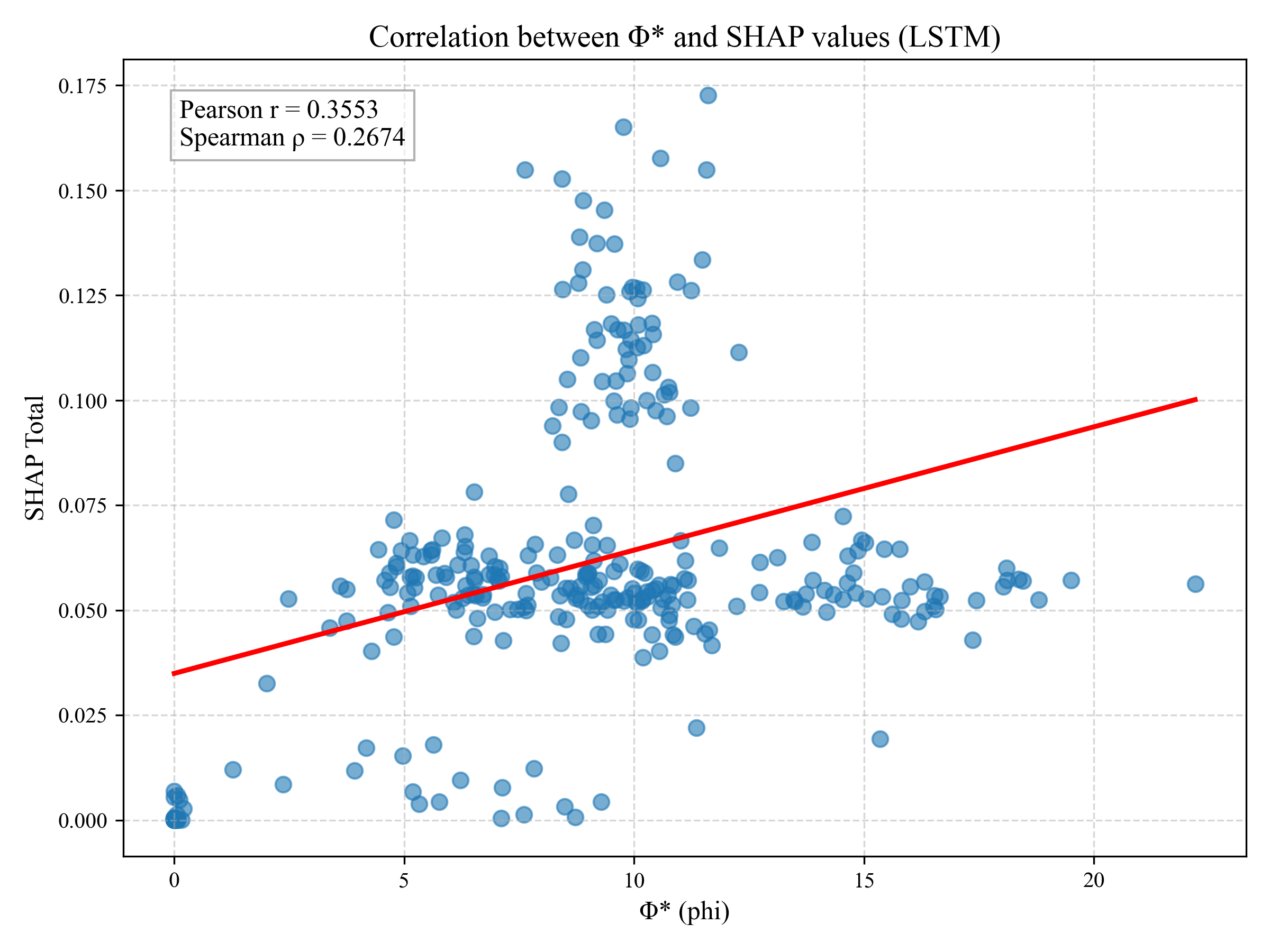
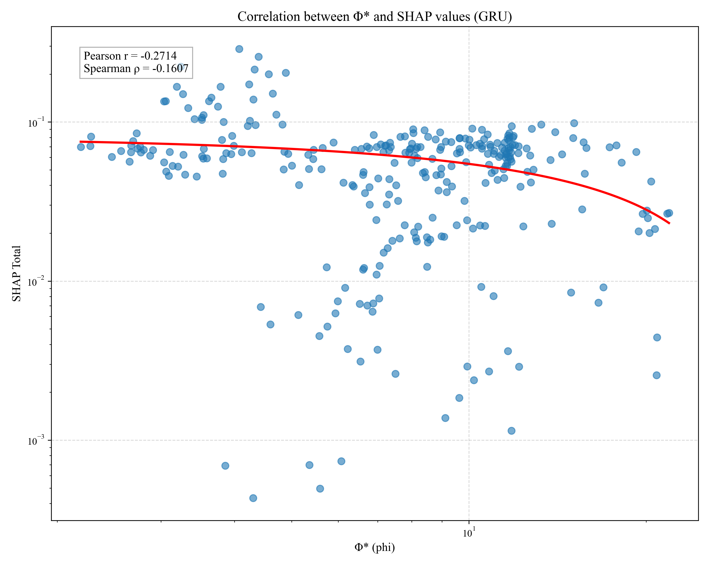
The relationship is architecture-dependent, hinting that gating may couple internal integration to feature attribution. Given the estimator floor and fragility documented above, these are reported as exploratory hypotheses, not established effects.

9Conclusion

Computation and integration are dissociable. Exact Φ makes this vivid: a feedforward network solves its task perfectly with Φ = 0, and rewiring alone — holding the task fixed — raises Φ to 2.47. The scalable results agree: architectures that all reach ceiling accuracy differ threefold in Φ*, and Φ* is statistically uncorrelated with accuracy. Under IIT this is expected, because Φ tracks intrinsic causal structure rather than input–output function.

But integration is not robustly measurable at useful scale. Exact Φ is intractable beyond about a dozen units. The scalable surrogate, Φ*, is a different quantity that has a non-zero floor, conflates integration with redundancy, and swings by factors of several with estimator settings; its cross-architecture ranking even reverses once settings are matched. Claims of the form "architecture X is the most integrated" are therefore not currently defensible from Φ*.

Together these give a specific answer to whether there is more to consciousness than computation: under IIT, yes — integration depends on causal organization, not on the computed function — but our present tools cannot measure that integration reliably in artificial systems.

10Reproduce

The phi_star_replication/ package contains the shared matched estimator, the multi-seed runner, the synthetic validation, the sensitivity analysis, and every result file and figure shown here.

Table 4. Package contents.
File	Purpose
`phi_star.py`	The shared, documented Φ* estimator.
`models.py`	Grammar task + RNN/GRU/LSTM and hidden-state collector.
`run_experiments.py`	Matched multi-seed training + Φ* tracking.
`validate_estimator.py`	Synthetic coupled vs. independent check.
`sensitivity.py`	How Φ* depends on estimator settings.
`analyze.py`	Aggregates seeds into figures and summary table.

Raw MNIST is not committed — it downloads automatically via torchvision. The recurrent tasks use synthetic data generated in code.

11Contact

Questions about the methods, the code, or the results? Send a message below.